Gurtaj's blog!

In this notebook I attempt to improve my result on my previous attempt of a CNN using nn.conv2d (see this notebook). I aim to do this by applying the concepts I learned when fixing my simple linear model (see this notebook).

TL;DR

Some key aspects of my learning when fixing this model were as follows:

cross-entropy was used as the loss function.
- previously I had always used RMSE (root mean squared error). But that is better for a linear regression. Here we have a classification problem and for this cross-entropy is much better suited.
- (the real reason why cross-entropy is used most often for classification problems, is that experience shows that it very often leads to better results)
nan values for valid_loss where occuring due to some of the predicted activations where 0 at the time of checking accuracy of an epoch.
- this was fixed by adding a small amount, pred = F.relu(pred), to each activation.
- prior to that F.relu was also used to get rid of any negative values which would also lead to nan values after use of torch.log in our mean_cross_entropy function.

# This Python 3 environment comes with many helpful analytics libraries installed
# It is defined by the kaggle/python Docker image: https://github.com/kaggle/docker-python
# For example, here's several helpful packages to load

import numpy as np # linear algebra
import pandas as pd # data processing, CSV file I/O (e.g. pd.read_csv)

# Input data files are available in the read-only "../input/" directory
# For example, running this (by clicking run or pressing Shift+Enter) will list all files under the input directory

import os
for dirname, _, filenames in os.walk('/kaggle/input'):
    for filename in filenames:
        print(os.path.join(dirname, filename))

# You can write up to 20GB to the current directory (/kaggle/working/) that gets preserved as output when you create a version using "Save & Run All" 
# You can also write temporary files to /kaggle/temp/, but they won't be saved outside of the current session

# install fastkaggle if not available
try: import fastkaggle
except ModuleNotFoundError:
    !pip install -Uq fastkaggle

from fastkaggle import *

comp = 'digit-recognizer'

path = setup_comp(comp, install='fastai "timm>=0.6.2.dev0"')

Warning: Your Kaggle API key is readable by other users on this system! To fix this, you can run 'chmod 600 /Users/gaz/.kaggle/kaggle.json'

from fastai.vision.all import *

path.ls()

(#3) [Path('digit-recognizer/test.csv'),Path('digit-recognizer/train.csv'),Path('digit-recognizer/sample_submission.csv')]

df = pd.read_csv(path/'train.csv')
df

	label	pixel0	pixel1	pixel2	pixel3	pixel4	pixel5	pixel6	pixel7	pixel8	...	pixel774	pixel775	pixel776	pixel777	pixel778	pixel779	pixel780	pixel781	pixel782	pixel783
0	1	0	0	0	0	0	0	0	0	0	...	0	0	0	0	0	0	0	0	0	0
1	0	0	0	0	0	0	0	0	0	0	...	0	0	0	0	0	0	0	0	0	0
2	1	0	0	0	0	0	0	0	0	0	...	0	0	0	0	0	0	0	0	0	0
3	4	0	0	0	0	0	0	0	0	0	...	0	0	0	0	0	0	0	0	0	0
4	0	0	0	0	0	0	0	0	0	0	...	0	0	0	0	0	0	0	0	0	0
...	...	...	...	...	...	...	...	...	...	...	...	...	...	...	...	...	...	...	...	...	...
41995	0	0	0	0	0	0	0	0	0	0	...	0	0	0	0	0	0	0	0	0	0
41996	1	0	0	0	0	0	0	0	0	0	...	0	0	0	0	0	0	0	0	0	0
41997	7	0	0	0	0	0	0	0	0	0	...	0	0	0	0	0	0	0	0	0	0
41998	6	0	0	0	0	0	0	0	0	0	...	0	0	0	0	0	0	0	0	0	0
41999	9	0	0	0	0	0	0	0	0	0	...	0	0	0	0	0	0	0	0	0	0

42000 rows × 785 columns

Data Preperation

Lets split this data into training and validation data.
We will split by rows.
We will use 80% for training and 20% for validation. 80% of 42,000 is 33,600 so that will be our split index.

train_data_split = df.iloc[:33_600,:]
valid_data_split = df.iloc[33_600:,:]

len(train_data_split)/42000,len(valid_data_split)/42000

(0.8, 0.2)

Our pixel values can be anywhere between 0 and 255. For good practice, and ease of use later, we’ll normalise all these values by dividing by 255 so that they are all values between 0 and 1.

pixel_value_columns = train_data_split.iloc[:,1:]
label_value_column = train_data_split.iloc[:,:1]

pixel_value_columns = pixel_value_columns.apply(lambda x: x/255)
train_data = pd.concat([label_value_column, pixel_value_columns], axis=1)

train_data.describe()

	label	pixel0	pixel1	pixel2	pixel3	pixel4	pixel5	pixel6	pixel7	pixel8	...	pixel774	pixel775	pixel776	pixel777	pixel778	pixel779	pixel780	pixel781	pixel782	pixel783
count	33600.000000	33600.0	33600.0	33600.0	33600.0	33600.0	33600.0	33600.0	33600.0	33600.0	...	33600.000000	33600.000000	33600.000000	33600.000000	33600.000000	33600.000000	33600.0	33600.0	33600.0	33600.0
mean	4.459881	0.0	0.0	0.0	0.0	0.0	0.0	0.0	0.0	0.0	...	0.000801	0.000454	0.000255	0.000086	0.000037	0.000007	0.0	0.0	0.0	0.0
std	2.885525	0.0	0.0	0.0	0.0	0.0	0.0	0.0	0.0	0.0	...	0.024084	0.017751	0.013733	0.007516	0.005349	0.001326	0.0	0.0	0.0	0.0
min	0.000000	0.0	0.0	0.0	0.0	0.0	0.0	0.0	0.0	0.0	...	0.000000	0.000000	0.000000	0.000000	0.000000	0.000000	0.0	0.0	0.0	0.0
25%	2.000000	0.0	0.0	0.0	0.0	0.0	0.0	0.0	0.0	0.0	...	0.000000	0.000000	0.000000	0.000000	0.000000	0.000000	0.0	0.0	0.0	0.0
50%	4.000000	0.0	0.0	0.0	0.0	0.0	0.0	0.0	0.0	0.0	...	0.000000	0.000000	0.000000	0.000000	0.000000	0.000000	0.0	0.0	0.0	0.0
75%	7.000000	0.0	0.0	0.0	0.0	0.0	0.0	0.0	0.0	0.0	...	0.000000	0.000000	0.000000	0.000000	0.000000	0.000000	0.0	0.0	0.0	0.0
max	9.000000	0.0	0.0	0.0	0.0	0.0	0.0	0.0	0.0	0.0	...	0.996078	0.996078	0.992157	0.992157	0.956863	0.243137	0.0	0.0	0.0	0.0

8 rows × 785 columns

Let’s further process our data so that it is ready for this new type of model we are using. Note that:

we will use 28*28 pixel matrices for our images rather than 783 pixel vectors
- because convolutions are done on matrices
we also add a dimension of 1 as the first dimension (view(1,28,28)) because Conv2d takes in ‘channels’ for each image, and it expects colour images
- colour images would have 3 channels, 1 for each colour (RGB).
- since we are only dealing with black and white images (one colour) we will deal with only one channel

pixel_value_columns = train_data_split.iloc[:,1:]
label_value_column = train_data_split.iloc[:,:1]

pixel_value_columns = pixel_value_columns.apply(lambda x: x/255)

pixel_value_columns_tensor = torch.tensor(train_data.iloc[:,1:].values).float()
# here we change from image vectors to image matrices and put it in our three channels (three channels since resnet18 expects 3 channel images (RGB))
pixel_value_matrices_tensor = [row.view(1,28,28) for row in pixel_value_columns_tensor]

label_value_column_tensor = torch.tensor(label_value_column.values).float()

# F.cross_entropy requires that the labels are tensor of scalar. label values cannot be `FloatTensor` if they are classes (discrete values), must be cast to `LongTensor` (`LongTensor` is synonymous with integer)
train_ds = list(zip(pixel_value_matrices_tensor, label_value_column_tensor.squeeze().type(torch.LongTensor)))

train_dl = DataLoader(train_ds, batch_size=256)

train_xb,train_yb = first(train_dl)

train_xb.shape,train_yb.shape

(torch.Size([256, 1, 28, 28]), torch.Size([256]))

We’ll make the above data-prep logic a function, so that we can do the same again for our validation data.

def dataloader_from_dataframe(dframe):
    pixel_value_columns = dframe.iloc[:,1:]
    label_value_column = dframe.iloc[:,:1]

    pixel_value_columns = pixel_value_columns.apply(lambda x: x/255)

    pixel_value_columns_tensor = torch.tensor(dframe.iloc[:,1:].values).float()
    # here we change from image vectors to image matrices and put it in our three channels (three channels since resnet18 expects 3 channel images (RGB))
    pixel_value_matrices_tensor = [row.view(1,28,28) for row in pixel_value_columns_tensor]

    label_value_column_tensor = torch.tensor(label_value_column.values).float()

    # F.cross_entropy requires that the labels are tensor of scalar. label values cannot be `FloatTensor` if they are classes (discrete values), must be cast to `LongTensor` (`LongTensor` is synonymous with integer)
    valid_ds = list(zip(pixel_value_matrices_tensor, label_value_column_tensor.squeeze().type(torch.LongTensor)))

    return DataLoader(valid_ds, batch_size=256)

valid_dl = dataloader_from_dataframe(valid_data_split)

valid_xb,valid_yb = first(valid_dl)

valid_xb.shape,valid_xb.shape

(torch.Size([256, 1, 28, 28]), torch.Size([256, 1, 28, 28]))

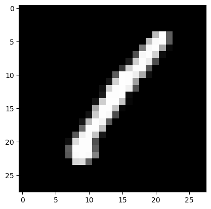
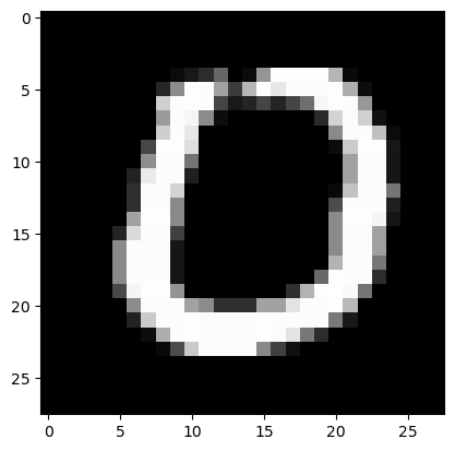
To ease my mind and help spot places where I could be making errors, i’ll make a function that can visually show a particular input (digit image) to me.

def show_image(item):
    plt.gray()
    plt.imshow(item, interpolation='nearest')
    plt.show()

Now, for my sanity, i’ll test an image in our prepped/re-formatted training data.

# we access the first (and only) channel of the first image of our first batch of training and validation data
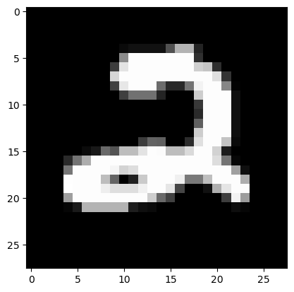
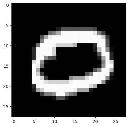
show_image(train_xb[0][0]),show_image(valid_xb[0][0])

png

(None, None)

Loss Function

Before calculating our loss, we will want to one-hot encode all our label values. This will correspond to our predictions which will have an acitivation/probability for each possible class (digit from 0-9).

number_of_classes = 10

def one_hot(yb):
    batch_size = len(yb)
    one_hot_yb = torch.zeros(batch_size, number_of_classes)
    x_coordinates_array = torch.arange(len(one_hot_yb))
    # used `.squeeze()` becasue yb originally has the size (batch_size, 1) and we just want a size of (batch_size). ([1, 2, 3, ...] instead of [[1], [2], [3], ...])
    # used `.long()` because: "tensors used as indices must be long, int, byte or bool tensors"
    y_coordinates_array = yb.squeeze().long()
    # set to `1.` rather than `1` because: Index put requires the source and destination dtypes match, got Float for the destination and Long for the source.
    one_hot_yb[x_coordinates_array, y_coordinates_array] = torch.tensor(1.)
    
    return one_hot_yb.T

one_hot(train_yb),one_hot(train_yb).shape,one_hot(train_yb)[:,0],train_yb[0]

(tensor([[0., 1., 0.,  ..., 0., 0., 0.],
         [1., 0., 1.,  ..., 0., 0., 1.],
         [0., 0., 0.,  ..., 0., 0., 0.],
         ...,
         [0., 0., 0.,  ..., 0., 1., 0.],
         [0., 0., 0.,  ..., 0., 0., 0.],
         [0., 0., 0.,  ..., 0., 0., 0.]]),
 torch.Size([10, 256]),
 tensor([0., 1., 0., 0., 0., 0., 0., 0., 0., 0.]),
 tensor(1))

Cross Entropy Loss

The function for cross entropy is as follows $H(p,q)=-\sum_{x}^{}p(x)\log q(x)$

$p(x)$ is the probability of $x$ in $p$ (the observed probability distribution) - in other words a value within label (0 or 1 in this case)
$q(x)$ is the probability of $x$ in $q$ (the predicted probability distribution) - in other words an activation in our prediction
NOTE that $H(p,q)\neq H(q,p)$ (the order matters).

Note how, since our label’s are going to be one-hot encoded, all values in the lable are going to be 0 apart from the one that corresponds to the correct digit which will be 1. So the calculation effectively is just going to become the negative of the log of the activation value (in our prediction) that corresponds to the correct digit.

Let’s try to recreate this in PyTorch.

def cross_entropy(pred, actual):
	actual = one_hot(actual.squeeze()).T
	
	return sum(actual * torch.log(pred))

I want to confirm that this is actually doing what we expect it to.

prd = torch.tensor([0.0977, 0.0985, 0.1010, 0.1011, 0.1051, 0.0970, 0.1027, 0.0987, 0.1007,
        0.0974])
one_ht_lbl = torch.tensor([0., 1., 0., 0., 0., 0., 0., 0., 0., 0.])

# index of non zero value in one hot coded label is 1
one_ht_lbl[1] * torch.log(prd[1]),sum(one_ht_lbl * torch.log(prd))

(tensor(-2.3177), tensor(-2.3177))

This clarifies that sum(one_ht_lbl * torch.log(prd)) does in fact do the element-wise product of the two inputs and then take the sum over all of them. Now what about when we are dealing with more than one prediction.

prds = torch.tensor([[0.0977, 0.0985, 0.1010, 0.1011, 0.1051, 0.0970, 0.1027, 0.0987, 0.1007,0.0974],[0.0977, 0.0985, 0.1010, 0.1011, 0.1051, 0.0970, 0.1027, 0.0987, 0.1007,0.0974],[0.0977, 0.0985, 0.1010, 0.1011, 0.1051, 0.0970, 0.1027, 0.0987, 0.1007,0.0974]])
one_ht_lbls = torch.tensor([[0., 1., 0., 0., 0., 0., 0., 0., 0., 0.],[0., 1., 0., 0., 0., 0., 0., 0., 0., 0.],[0., 1., 0., 0., 0., 0., 0., 0., 0., 0.]])

sum(one_ht_lbls * torch.log(prds))

tensor([ 0.0000, -6.9531,  0.0000,  0.0000,  0.0000,  0.0000,  0.0000,  0.0000,
         0.0000,  0.0000])

This is not what we want. This is an ouput of 10 values, but we want just one return value from our loss function. In that case we should take the entropy of each prediction and output the mean of all those entropies (this is what PyTorch’s pre-made functions, F.cross_entropy and torch.nn.CrossEntropyLoss, do by default too).

nmbr_of_prds = prds.shape[0]
ttl_entropy = 0
for i in range(nmbr_of_prds):
	ttl_entropy += sum(one_ht_lbls[i] * torch.log(prds[i]))
mean_entrpy = ttl_entropy/nmbr_of_prds

ttl_entropy,mean_entrpy

(tensor(-6.9531), tensor(-2.3177))

I realised that my earlier mistake which was producing the 10 outputs was the fact that I was using sum rather than torch.sum. so this can be simplified to what I was trying originally but with the correct function.

torch.sum(one_ht_lbls * torch.log(prds)),torch.sum(one_ht_lbls * torch.log(prds))/nmbr_of_prds

(tensor(-6.9531), tensor(-2.3177))

That’s more like it! So let’s create mean_cross_entropy as our loss function instead.

def mean_cross_entropy(pred, actual):
	number_of_preds = pred.shape[0]
	actual = one_hot(actual.squeeze()).T

	# get rid of all negative values because log of a negative (in our return value) is going to be undefined
	pred = F.relu(pred)
	# create a small value to add to our pred to make sure it is non zero - becaues log of zero is also undefined
	eps=1e-7
	pred = pred + eps
	
	return - torch.sum(actual * torch.log(pred))/number_of_preds

mean_cross_entropy(prds, torch.tensor([[1],[1],[1]]))

tensor(2.3177)

Let’s also check the case where we have 0 value activations in our preds.

zero_prds = torch.tensor([[0, 0, 0, 0, 0, 0, 0, 0, 0, 1],[0.0977, 0.0985, 0.1010, 0.1011, 0.1051, 0.0970, 0.1027, 0.0987, 0.1007,0.0974],[0.0977, 0.0985, 0.1010, 0.1011, 0.1051, 0.0970, 0.1027, 0.0987, 0.1007,0.0974]])

mean_cross_entropy(zero_prds, torch.tensor([[1],[1],[1]]))

tensor(6.9178)

Trainability

This is all going to be handled by fastai’s SGD. This is the optimisation function that we are going to use in our Learner

Validation and Metric

Training all be done via our Learner and the optimisation function that we choose. In this case we will be choosing SGD.

Accuracy Metric

Let’s first create a function that returns the specific class (digit) that each prediction (set of 10 probabilities) corresponds to.

def get_predicted_label(pred):
    #returns index of highest value in tensor, which convenietnly also is directly the the digit/label that it corresponds to
    return torch.argmax(pred)

get_predicted_label(torch.tensor([0,4,3,2,6,1]))

tensor(4)

Now we can check accuracy by comparing the predicted class to what the actual class is.

def batch_accuracy(preds, yb):
    preds = torch.tensor([get_predicted_label(pred) for pred in preds])
    # is_correct is a tensor of True and False values
    is_correct = preds==yb.squeeze()
    
    # now we turn all True values into 1 and all False values into 0, then return the mean of those values
    return is_correct.float().mean()

Conv2d

We are going to use the nn.Conv2d convolutional method provided by PyTorch. Along with that we will use Pytorch’s F.cross_entropy as the loss function and, as with the models in my previous notebooks, we’ll use SGD as our optimiser.

dls = DataLoaders(train_dl,valid_dl)

As stated earlier, we have a batch size of 256 of single-channel (1) images of size 28*28.

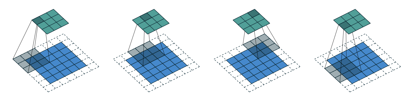
let’s try out a kernel size of 3.

Note kernels are a key part of convolutions:

they are a matrix of weights that essentially scans across the whole image and
for each of it’s positions we take an element-wise multiplication which is:
- the sum
- of each of the products
- of each of it’s weights,
- and each of the the pixels it is covering
an activation is produced for each kernal position and a new matrix is produced as a result.

Look up Chapter 13 Convolutions in fastai’s fastbook for more information.

ks=3

simple_conv_net = nn.Sequential(
    nn.Conv2d(1,30, kernel_size=ks, padding=1),
    nn.ReLU(),
    nn.Conv2d(30,10, kernel_size=ks, padding=1),
    nn.Softmax()
)

Lets see what shape our output will have with this model.

simple_conv_net(train_xb).shape

/Users/gaz/mambaforge/envs/fastbook/lib/python3.10/site-packages/torch/nn/modules/container.py:217: UserWarning: Implicit dimension choice for softmax has been deprecated. Change the call to include dim=X as an argument.
  input = module(input)

torch.Size([256, 10, 28, 28])

This is not something we can use to do classification, since we need a single output activation per image, not a 28×28 map of activations. One way to deal with this is to use enough stride-2 convolutions, and padding of 1, such that the final layer is size 10.

Stride is the amount of pixels that the kernel moves by after each position. And the general formula for resultant matrix size is (n + 2*pad - ks)//stride + 1 where pad is the padding, stride is the stride and ks is the kernel size. stride-2 convolutions are useful for decreasing the size of our outputs, and stride-1 convolutions are useful for adding layers without changing the output size

Padding is number of pixels added to the outside of our image. Without padding, and with a stride-1 (no change in output size due to slide) the output matrix will lose size on each dimension. This is due to the fact that the kernel will not go boyond the edges of the image itself. We can counteract this by adding padding. The necessary padding on each side to keep the same shape is ks//2. (see image below that shows how the image can move further with a padding of 2 added)

With some experimentation I found an architecture that gives the desired output format.

simple_conv_net = nn.Sequential(
    nn.Conv2d(1,4, stride=2, kernel_size=ks, padding=ks//2), 
    nn.ReLU(),
    nn.Conv2d(4,16, stride=2, kernel_size=ks, padding=ks//2),
    nn.ReLU(),
    nn.Conv2d(16,32, stride=2, kernel_size=ks, padding=ks//2),
    nn.ReLU(),
    nn.Conv2d(32,64, stride=2, kernel_size=ks, padding=ks//2),
    nn.ReLU(),
    nn.Conv2d(64,10, stride=2, kernel_size=ks, padding=ks//2),
    nn.Flatten(),
    nn.Softmax(dim=1)
)

simple_conv_net(train_xb).shape,sum(simple_conv_net(train_xb)[0])

(torch.Size([256, 10]), tensor(1.0000, grad_fn=<AddBackward0>))

10 activations/outputs, one for each class (digit), just what we wanted!

Note how the only thing I adapted in the end was the number of layers and the number of channels in and out in each layer.

You will Also notice that I used nn.Flatten. This is becuase out output shape was actually [256, 10, 1, 1] so to remove those extra [1, 1] axis we used Flatten. It is basically the same as PyTorch’s squeeze method but as a PyTorch module instead. And as we’ve seen previously we used nn.Softmax to make sure that our 10 activations per image add up to 1.

Now we can give this model a try.

learn = Learner(dls, simple_conv_net, opt_func=SGD,
                loss_func=mean_cross_entropy, metrics=batch_accuracy)

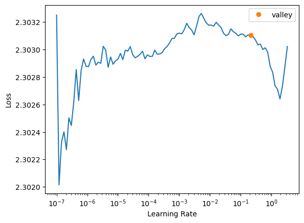
learn.lr_find()

SuggestedLRs(valley=0.2089296132326126)

png

learn.fit_one_cycle(n_epoch=10, lr_max = 0.2)

epoch	train_loss	valid_loss	batch_accuracy	time
0	2.302217	2.333876	0.112143	00:13
1	2.300602	2.334830	0.115952	00:14
2	2.226018	9.240983	0.405595	00:14
3	0.550190	1.504575	0.905357	00:13
4	0.213293	1.113232	0.929762	00:13
5	0.142037	0.857645	0.945952	00:13
6	0.113845	0.622772	0.960476	00:14
7	0.098793	0.541029	0.966071	00:14
8	0.090647	0.517730	0.967381	00:14
9	0.087030	0.511101	0.967738	00:14

The numbers don’t look too bad but I am still sceptical due to past experiences! We will now run this on the competition test data and see how it performs on the leaderboard.

Getting Predictions on the Test Data

Lets first format our test data in the same way that we formated our training data, as this is what our model is expecting.

path.ls()

(#3) [Path('digit-recognizer/test.csv'),Path('digit-recognizer/train.csv'),Path('digit-recognizer/sample_submission.csv')]

test_df = pd.read_csv(path/'test.csv')

test_df

	pixel0	pixel1	pixel2	pixel3	pixel4	pixel5	pixel6	pixel7	pixel8	pixel9	...	pixel774	pixel775	pixel776	pixel777	pixel778	pixel779	pixel780	pixel781	pixel782	pixel783
0	0	0	0	0	0	0	0	0	0	0	...	0	0	0	0	0	0	0	0	0	0
1	0	0	0	0	0	0	0	0	0	0	...	0	0	0	0	0	0	0	0	0	0
2	0	0	0	0	0	0	0	0	0	0	...	0	0	0	0	0	0	0	0	0	0
3	0	0	0	0	0	0	0	0	0	0	...	0	0	0	0	0	0	0	0	0	0
4	0	0	0	0	0	0	0	0	0	0	...	0	0	0	0	0	0	0	0	0	0
...	...	...	...	...	...	...	...	...	...	...	...	...	...	...	...	...	...	...	...	...	...
27995	0	0	0	0	0	0	0	0	0	0	...	0	0	0	0	0	0	0	0	0	0
27996	0	0	0	0	0	0	0	0	0	0	...	0	0	0	0	0	0	0	0	0	0
27997	0	0	0	0	0	0	0	0	0	0	...	0	0	0	0	0	0	0	0	0	0
27998	0	0	0	0	0	0	0	0	0	0	...	0	0	0	0	0	0	0	0	0	0
27999	0	0	0	0	0	0	0	0	0	0	...	0	0	0	0	0	0	0	0	0	0

28000 rows × 784 columns

Unlike our training data, this data has no label values so we will make a slightly modified version of our dataloader_from_dataframe that doesn’t split the data into pixel values and label values. And we’ll just use a bunch of 0s for our lavel values instead. They’re not going to actually be used as we are only using this data to make predictions, not for training or validation. We just need to add them for the sake of what is expected of a DataLoader by fastai.

Note taht the reason we convert it into a DataLoader is because we are going to use learn.get_preds to get our predictions, which expects the input in that format.

def dataloader_from_test_dataframe(dframe):
    pixel_value_columns_tensor = torch.tensor(dframe.values).float()
    # here we change from image vectors to image matrices and put it in our three channels (three channels since resnet18 expects 3 channel images (RGB))
    pixel_value_matrices_tensor = [row.view(1,28,28) for row in pixel_value_columns_tensor]

    dummy_label_value_column_tensor = torch.zeros(len(pixel_value_columns_tensor)).float()

    # F.cross_entropy requires that the labels are tensor of scalar. label values cannot be `FloatTensor` if they are classes (discrete values), must be cast to `LongTensor` (`LongTensor` is synonymous with integer)
    ds = list(zip(pixel_value_matrices_tensor, dummy_label_value_column_tensor.squeeze().type(torch.LongTensor)))

    return DataLoader(ds, batch_size=len(pixel_value_columns_tensor))

test_dl = dataloader_from_test_dataframe(test_df)

test_xb,test_yb = first(test_dl)
test_xb.shape,test_yb.shape

(torch.Size([28000, 1, 28, 28]), torch.Size([28000]))

show_image(test_xb[0][0]),show_image(test_xb[1][0])

png

(None, None)

preds = learn.get_preds(dl=test_dl)

preds_x,labels_y = preds
preds_x[0],labels_y[0],preds_x[1],labels_y[1]

(tensor([0., 0., 1., 0., 0., 0., 0., 0., 0., 0.]),
 tensor(0),
 tensor([1., 0., 0., 0., 0., 0., 0., 0., 0., 0.]),
 tensor(0))

These are corresponding very nicely to the actual images which we previewed above (using our show_image function).
Note how the lables are always 0, this is just the dummy labels we added when creating our DataLoader (test_dl).

Submitting Results

let’s look at our submission example

ss = pd.read_csv(path/'sample_submission.csv')

ss

	ImageId	Label
0	1	0
1	2	0
2	3	0
3	4	0
4	5	0
...	...	...
27995	27996	0
27996	27997	0
27997	27998	0
27998	27999	0
27999	28000	0

28000 rows × 2 columns

Of course the labels are exepected to be single values, so let’s convert our outputted precitions/activations into the classes they correspond too.

pred_labels = [get_predicted_label(pred).numpy() for pred in preds_x]

pred_labels[:5]

[array(2), array(0), array(9), array(9), array(3)]

Now we simply need to replace the blank labels with our predicted ones (see competition guidlines).

ss['Label'] = pred_labels

ss

	ImageId	Label
0	1	2
1	2	0
2	3	9
3	4	9
4	5	3
...	...	...
27995	27996	9
27996	27997	7
27997	27998	3
27998	27999	9
27999	28000	2

28000 rows × 2 columns

Looks good! now we can submit this to kaggle.

We can do it straight from this note book if we are running it on Kaggle, otherwise we can use the API
In this case I was using this notebook in my IDE so I submitted via the API.

# this outputs the actual file
ss.to_csv('subm.csv', index=False)
#this shows the head (first few lines)
!head subm.csv

ImageId,Label
1,2
2,0
3,9
4,9
5,3
6,7
7,0
8,3
9,0

!kaggle competitions submit -c digit-recognizer  -f ./subm.csv -m "conv2d network with cross-entropy loss"

After submitting the results, a score of 0.9676 was receivied, the best score I’ve acheived on this competition to date!

Conclusion

Clearly the thing’s I have learned about importance of the shape of the data throughout our model, and the choice of loss function, were very crucial in getting this model to work properly. Even though I had it running previously, it clearly was not doing what I had intended it to do!

In the words of Jeremy Howard:

The stuff in the middle of the model you’re note going to have to care about much in your life, if ever. But the stuff that happens in the first layer and the last layer, including the loss function that sits between the last layer and the loss, you’re gonna have to care about a lot.

I saw this in my experience here, with the selection of the cross-entropy function as the loss function and then having to ensure that it could handle all posible values given to it as well.