Gurtaj's blog!
Introduction
After not being able to successfully produce a linear model previously (see this notebook), I decided to go all the way down to basics to see what I was missing (see this notebook). I actually came to recognise that, during the process of a model in training, a lot more data augmentation took place that I first thought.
In this notebook I aim to see if any of this new found knowledge can help to improve what I had made in my previous linear model attempt.
The notebook below details my efforts. Note that I did not include the explanations from the original notebook, only explanations on anything I changed or discovered.
TL;DR
The places where I was going wrong previously were as follows
- I was previously making one measurement/prediction per image
- In the end this is what we want but for the interim (traning and accuracy determination) it helps to have one output for each class we are trying to distinguish between (10 classes for digits 0-9)
- The shape of my data at each step matters more than I realised. The matrix multiplications as well as simple things like subtraction and mean, all require care and attention to detail to ensure that the data is in the correct format. Having data in the wrong format does not always mean that an error will be thrown and this is why these things can cause big issues further down the line without us even becoming aware of what is causing them (as was the case for me in my accuracy calcuations)
# This Python 3 environment comes with many helpful analytics libraries installed
# It is defined by the kaggle/python Docker image: https://github.com/kaggle/docker-python
# For example, here's several helpful packages to load

import numpy as np # linear algebra
import pandas as pd # data processing, CSV file I/O (e.g. pd.read_csv)

# Input data files are available in the read-only "../input/" directory
# For example, running this (by clicking run or pressing Shift+Enter) will list all files under the input directory

import os
for dirname, _, filenames in os.walk('/kaggle/input'):
    for filename in filenames:
        print(os.path.join(dirname, filename))

# You can write up to 20GB to the current directory (/kaggle/working/) that gets preserved as output when you create a version using "Save & Run All"
# You can also write temporary files to /kaggle/temp/, but they won't be saved outside of the current session
# install fastkaggle if not available
try: import fastkaggle
except ModuleNotFoundError:
    !pip install -Uq fastkaggle

from fastkaggle import *
comp = 'digit-recognizer'

path = setup_comp(comp, install='fastai "timm>=0.6.2.dev0"')
from fastai.vision.all import *
path.ls()
(#3) [Path('digit-recognizer/test.csv'),Path('digit-recognizer/train.csv'),Path('digit-recognizer/sample_submission.csv')]
df = pd.read_csv(path/'train.csv')
df
Data Preparation
train_data_split = df.iloc[:33_600,:]
valid_data_split = df.iloc[33_600:,:]

len(train_data_split)/42000,len(valid_data_split)/42000
pixel_value_columns = train_data_split.iloc[:,1:]
label_value_column = train_data_split.iloc[:,:1]

pixel_value_columns = pixel_value_columns.apply(lambda x: x/255)
train_data = pd.concat([label_value_column, pixel_value_columns], axis=1)

train_data.describe()
pixel_value_columns_tensor = torch.tensor(train_data.iloc[:,1:].values).float()
label_value_column_tensor = torch.tensor(train_data.iloc[:,:1].values).float()

train_ds = list(zip(pixel_value_columns_tensor,label_value_column_tensor))
We’ll make this a function, so that we can do the same again for our validation data.
train_dl = DataLoader(train_ds, batch_size=256)
train_xb,train_yb = first(train_dl)

train_xb.shape,train_xb.shape
(torch.Size([256, 784]), torch.Size([256, 784]))
def dataset_from_dataframe(dframe):
    pixel_value_columns = dframe.iloc[:,1:]
    label_value_column = dframe.iloc[:,:1]

    pixel_value_columns = pixel_value_columns.apply(lambda x: x/255)

    pixel_value_columns_tensor = torch.tensor(train_data.iloc[:,1:].values).float()
    label_value_column_tensor = torch.tensor(train_data.iloc[:,:1].values).float()

    return list(zip(pixel_value_columns_tensor, label_value_column_tensor))
valid_ds = dataset_from_dataframe(valid_data_split)

valid_dl = DataLoader(valid_ds, batch_size=256)
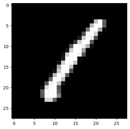
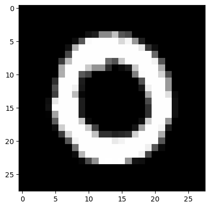
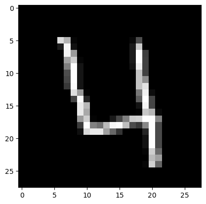
To ease my mind and help spot places where I could be making errors, i’ll make a function that can visually show a particular input (digit image) to me.
def show_image(item):
    item = item.view(28,28) * 255
    plt.gray()
    plt.imshow(item, interpolation='nearest')
    plt.show()
Now, for my sanity, i’ll test a few images in train_xb.
show_image(train_xb[0])
show_image(train_xb[1])
show_image(train_xb[3])
def init_params(size): return (torch.rand(size) - 0.5).requires_grad_()
So this is the furst place that I realised what I had done before was wrong.
Previously I was producing just one prediction per image. We actually want 10 predictions for each image (it’s likelyhood of being each of the digits from 0-9), so we will now have 10 set’s of weights and 10 biases.
weights = init_params((10,784))
bias = init_params((10,1))
weights.shape,bias.shape,train_xb[0].shape
(torch.Size([10, 784]), torch.Size([10, 1]), torch.Size([784]))
Let’s create our batch linear function.
W do this just as before, but now we will transpose our batch so that our matrix multiplcation (@ below) will have the dimensions of the items on either side of it, in the correct order.
def linear(batch): return weights@batch.T + bias
first_batch_predictions = linear(train_xb)

first_batch_predictions,first_batch_predictions.shape
(tensor([[-2.3896, -0.1935, -2.7594,  ..., -0.1530, -0.9728,  0.2415],
         [-1.3769, -2.5199, -1.9325,  ..., -1.0211, -1.6149, -1.6244],
         [-1.6542, -2.7221,  1.2733,  ...,  3.3614,  2.6375, -1.3591],
         ...,
         [-1.2527,  6.4562,  0.5795,  ...,  4.6149, -0.1018, -1.1624],
         [-0.6726,  0.3058,  2.7778,  ...,  0.0544, -0.5529, -0.9122],
         [-3.7061, -1.4103, -3.6473,  ..., -6.0080, -5.5166, -0.2390]],
        grad_fn=<AddBackward0>),
 torch.Size([10, 256]))
Note how we are producing an output of 10 values (per image). We are doing this because we have 10 classes for which we are checking against. Our model should tell us which of those classes it is most likely that an input could be.
Later, we will one-hot encode all our Y-values. This means each label value in Y will be an array of 10 values, where all values are 0 apart from the one on the relevant index that will be 1. The relevant index will correspond to the digit that the label denotes. So, for example, a label of 4 will be come a one hot encoded array of [0,0,0,0,1,0,0,0,0,0]. The 1 appears at the 4th index in the array. The shape of our one-hot encoded labels will correspond to the shape of our predictions, which will be needed for our loss function.
So what we also want to do is make sure each of our 10 output values of our model are values between 0 and 1 (with their total being 1). We can do that by running it through the soft max equation. Let’s update linear to include that.
def linear(batch):
    res = weights@batch.T + bias

    return F.softmax(res, dim=0)
first_batch_predictions = linear(train_xb)

first_batch_predictions,first_batch_predictions.shape
(tensor([[2.1292e-02, 1.2629e-03, 1.4275e-03,  ..., 1.9981e-03, 3.4236e-03,
          1.4774e-01],
         [5.8615e-02, 1.2332e-04, 3.2637e-03,  ..., 8.3868e-04, 1.8015e-03,
          2.2864e-02],
         [4.4421e-02, 1.0074e-04, 8.0538e-02,  ..., 6.7131e-02, 1.2660e-01,
          2.9811e-02],
         ...,
         [6.6366e-02, 9.7566e-01, 4.0241e-02,  ..., 2.3511e-01, 8.1801e-03,
          3.6290e-02],
         [1.1855e-01, 2.0808e-03, 3.6255e-01,  ..., 2.4587e-03, 5.2104e-03,
          4.6607e-02],
         [5.7075e-03, 3.7406e-04, 5.8751e-04,  ..., 5.7258e-06, 3.6405e-05,
          9.1379e-02]], grad_fn=<SoftmaxBackward0>),
 torch.Size([10, 256]))
Let’s see what we get from the first column (results of the first image).
first_batch_predictions[:,0]
tensor([0.0213, 0.0586, 0.0444, 0.3606, 0.0220, 0.2023, 0.1001, 0.0664, 0.1185,
        0.0057], grad_fn=<SelectBackward0>)
Just to confirm that we did the softmax call across the right dimenstion, let’s ensure all these 10 values now add up to 1.
sum(first_batch_predictions[:,0])
tensor(1.0000, grad_fn=<AddBackward0>)
Loss Function
def rmse(a, b):
    mse = nn.MSELoss()
    loss = torch.sqrt(mse(a, b))

    return loss
As mentioned earlier, we need to one-hot encode all our Y values. So that we can compare them to our 10-value predictions (each value corresponds to the likelyhood of being one of the 10 possible digits).
number_of_classes = 10

def one_hot(yb):
    batch_size = len(yb)
    one_hot_yb = torch.zeros(batch_size, number_of_classes)
    x_coordinates_array = torch.arange(len(one_hot_yb))
    # used `.squeeze()` becasue yb originally has the size (batch_size, 1) and we just want a size of (batch_size). ([1, 2, 3, ...] instead of [[1], [2], [3], ...])
    # used `.long()` because: "tensors used as indices must be long, int, byte or bool tensors"
    y_coordinates_array = yb.squeeze().long()
    # set to `1.` rather than `1` because: Index put requires the source and destination dtypes match, got Float for the destination and Long for the source.
    one_hot_yb[x_coordinates_array, y_coordinates_array] = torch.tensor(1.)

    return one_hot_yb.T
one_hot(train_yb),one_hot(train_yb).shape,one_hot(train_yb)[:,0],train_yb[0]
(tensor([[0., 1., 0.,  ..., 0., 0., 0.],
         [1., 0., 1.,  ..., 0., 0., 1.],
         [0., 0., 0.,  ..., 0., 0., 0.],
         ...,
         [0., 0., 0.,  ..., 0., 1., 0.],
         [0., 0., 0.,  ..., 0., 0., 0.],
         [0., 0., 0.,  ..., 0., 0., 0.]]),
 torch.Size([10, 256]),
 tensor([0., 1., 0., 0., 0., 0., 0., 0., 0., 0.]),
 tensor([1.]))
Let’s run it on our test batch predictions from above.
rmse(first_batch_predictions, one_hot(train_yb))
tensor(0.3545, grad_fn=<SqrtBackward0>)
Trainability
def calc_grad(batch_inputs, batch_labels, batch_model):
    batch_preds = batch_model(batch_inputs)
    loss = rmse(batch_preds, one_hot(batch_labels))
    loss.backward()
def train_epoch(dl, batch_model, params, lr):
    for xb,yb in dl:
        calc_grad(xb, yb, batch_model)
        for p in params:
            pdata1 = p.data
            p.data -= p.grad*lr
            pdata2 = p.data
            p.grad.zero_()
Validation and Metric
def get_predicted_label(pred):
    #returns index of highest value in tensor, which convenietnly also is directly the the digit/label that it corresponds to
    return torch.argmax(pred)
get_predicted_label(torch.tensor([0,4,3,2,6,1]))
tensor(4)
Let’s test this on some predictions from first_batch_predictions to ensure that we are getting sensible values (values from 0-9)
get_predicted_label(first_batch_predictions[:,0]),get_predicted_label(first_batch_predictions[:,1]),get_predicted_label(first_batch_predictions[:,3]),get_predicted_label(first_batch_predictions[:,5]),get_predicted_label(first_batch_predictions[:,33])
(tensor(3), tensor(7), tensor(7), tensor(7), tensor(4))
Accuracy
I, after far too long, decided that the model code, and optimisation code, were now all ok. So then I went on to look at batch_accuracy and this was where I found another issue that was causing me pain during the examination of my new code updates thus far!
look below at how it was before my final fix.
def batch_accuracy(preds, yb):
    #remember each column in our preds is an indivudual prediction, so we transpose preds in order to iterate through each precition in our list comprehension below
    preds = torch.tensor([get_predicted_label(pred) for pred in preds.T])
    # is_correct is a tensor of True and False values
    is_correct = preds==yb
    # now we turn all True values into 1 and all False values into 0, then return the mean of those values
    return is_correct.float().mean()
batch_accuracy(linear(train_xb[:100]),train_yb[:100])
tensor(0.0878)
What I didn’t realise was that, in my run above, preds had a shape of [100] whereas yb had a shape of [100, 1]. See below why this causes issues.
tensor([1,2,5]) == tensor([[1],[3],[5]])
tensor([[ True, False, False],
        [False, False, False],
        [False, False,  True]])
tensor([1,2,5]) == tensor([1,3,5])
tensor([ True, False, True])
So what was happening was that each prediction in preds, was being compared to, not only its corresponding label value, but all label values in yb, resulting in a tensor of shape [100, 100] rathen than just [100].
And then mean was taking the mean across each row and then returning the mean of those values! (See demonstrationd of how .mean() works below.
row1_mean = tensor([ True, False, False]).float().mean()
row2_mean = tensor([False, False, False]).float().mean()
row3_mean = tensor([False, False,  True]).float().mean()
mean_across_all_rows = (row1_mean+row2_mean+row3_mean)/3

total_mean = tensor([[ True, False, False],
        [False, False, False],
        [False, False,  True]]).float().mean()

row1_mean, row2_mean, row3_mean, mean_across_all_rows, total_mean
(tensor(0.3333), tensor(0.), tensor(0.3333), tensor(0.2222), tensor(0.2222))
So to get yb to the correct shape of [100] we can use the .squeeze() function. See demonstration below.
tensor([[1],[3],[5]]).squeeze()
tensor([1, 3, 5])
So let’s go ahead and update batch_accuracy.
def batch_accuracy(preds, yb):
    #remember each column in our preds is an indivudual prediction, so we transpose preds in order to iterate through each precition in our list comprehension below
    preds = torch.tensor([get_predicted_label(pred) for pred in preds.T])
    # is_correct is a tensor of True and False values
    # squeeze yb to correct shape
    is_correct = preds==yb.squeeze()
    # now we turn all True values into 1 and all False values into 0, then return the mean of those values
    return is_correct.float().mean()
batch_accuracy(linear(train_xb[:100]),train_yb[:100])
tensor(0.0700)
def validate_epoch(dl, batch_model):
    accuracies = [batch_accuracy(batch_model(xb),yb) for xb,yb in dl]
    # turn list of tensors into one single tensor of stacked values, so that we can then calculate the mean across all those values
    stacked_tensor = torch.stack(accuracies)
    mean_tensor = stacked_tensor.mean()
    # round method only works on value within tensor so we use item() to get it (and then round to four decimal places)
    return round(mean_tensor.item(), 4)
validate_epoch(valid_dl, linear)
0.1282
Train for Number of Epochs
lr = 0.01
params = weights,bias
train_epoch(train_dl, linear, params, lr)
validate_epoch(valid_dl, linear)
0.1351
Now let’s attempt at training our model over 500 more epochs and see if it improves.
for i in range(500):
    train_epoch(train_dl, linear, params, lr)
    # run validate_epoch on every 50th iteration
    if i % 50 == 0:
        print(validate_epoch(valid_dl, linear), ' ')
0.1433
0.4603
0.6433
0.7365
0.7875
0.8198
0.8398
0.8553
0.8651
0.8743
An ~87% accuracy on our validation data. I’ll now run this on the test data and submit it to the kaggle competition in order to see if it’s any good…
Competition Submission
test_df = pd.read_csv(path/'test.csv')

test_df.describe()
| pixel0 | pixel1 | pixel2 | pixel3 | pixel4 | pixel5 | pixel6 | pixel7 | pixel8 | pixel9 | ... | pixel774 | pixel775 | pixel776 | pixel777 | pixel778 | pixel779 | pixel780 | pixel781 | pixel782 | pixel783 | |
|---|---|---|---|---|---|---|---|---|---|---|---|---|---|---|---|---|---|---|---|---|---|
| count | 28000.0 | 28000.0 | 28000.0 | 28000.0 | 28000.0 | 28000.0 | 28000.0 | 28000.0 | 28000.0 | 28000.0 | ... | 28000.000000 | 28000.000000 | 28000.000000 | 28000.000000 | 28000.000000 | 28000.0 | 28000.0 | 28000.0 | 28000.0 | 28000.0 |
| mean | 0.0 | 0.0 | 0.0 | 0.0 | 0.0 | 0.0 | 0.0 | 0.0 | 0.0 | 0.0 | ... | 0.164607 | 0.073214 | 0.028036 | 0.011250 | 0.006536 | 0.0 | 0.0 | 0.0 | 0.0 | 0.0 |
| std | 0.0 | 0.0 | 0.0 | 0.0 | 0.0 | 0.0 | 0.0 | 0.0 | 0.0 | 0.0 | ... | 5.473293 | 3.616811 | 1.813602 | 1.205211 | 0.807475 | 0.0 | 0.0 | 0.0 | 0.0 | 0.0 |
| min | 0.0 | 0.0 | 0.0 | 0.0 | 0.0 | 0.0 | 0.0 | 0.0 | 0.0 | 0.0 | ... | 0.000000 | 0.000000 | 0.000000 | 0.000000 | 0.000000 | 0.0 | 0.0 | 0.0 | 0.0 | 0.0 |
| 25% | 0.0 | 0.0 | 0.0 | 0.0 | 0.0 | 0.0 | 0.0 | 0.0 | 0.0 | 0.0 | ... | 0.000000 | 0.000000 | 0.000000 | 0.000000 | 0.000000 | 0.0 | 0.0 | 0.0 | 0.0 | 0.0 |
| 50% | 0.0 | 0.0 | 0.0 | 0.0 | 0.0 | 0.0 | 0.0 | 0.0 | 0.0 | 0.0 | ... | 0.000000 | 0.000000 | 0.000000 | 0.000000 | 0.000000 | 0.0 | 0.0 | 0.0 | 0.0 | 0.0 |
| 75% | 0.0 | 0.0 | 0.0 | 0.0 | 0.0 | 0.0 | 0.0 | 0.0 | 0.0 | 0.0 | ... | 0.000000 | 0.000000 | 0.000000 | 0.000000 | 0.000000 | 0.0 | 0.0 | 0.0 | 0.0 | 0.0 |
| max | 0.0 | 0.0 | 0.0 | 0.0 | 0.0 | 0.0 | 0.0 | 0.0 | 0.0 | 0.0 | ... | 253.000000 | 254.000000 | 193.000000 | 187.000000 | 119.000000 | 0.0 | 0.0 | 0.0 | 0.0 | 0.0 |
8 rows × 784 columns
Now we format it into what our model expects. Since we don’t have labels for this data we’ll make a batch of inputs only (the batch will be the whole of the test data)
test_tensor = torch.tensor(test_df.values)/255

test_tensor.shape
torch.Size([28000, 784])
Now let’s create a function that produces a meaningful output (digit prediction) for each image, using our model.
def predict(batch):
    preds = linear(batch)
    # convert tensor to numpy value
    preds = [get_predicted_label(pred).numpy() for pred in preds.T]

    return preds
preds = predict(test_tensor)

preds[:5]
[array(2), array(0), array(9), array(7), array(3)]
pred_labels_series = pd.Series(preds, name="Label")

pred_labels_series
0        2
1        0
2        9
3        7
4        3
        ..
27995    9
27996    7
27997    3
27998    9
27999    2
Name: Label, Length: 28000, dtype: object
sample_submission = pd.read_csv(path/'sample_submission.csv')
sample_submission
| ImageId | Label | |
|---|---|---|
| 0 | 1 | 0 |
| 1 | 2 | 0 |
| 2 | 3 | 0 |
| 3 | 4 | 0 |
| 4 | 5 | 0 |
| ... | ... | ... |
| 27995 | 27996 | 0 |
| 27996 | 27997 | 0 |
| 27997 | 27998 | 0 |
| 27998 | 27999 | 0 |
| 27999 | 28000 | 0 |
28000 rows × 2 columns
len(test_df)
28000
sample_submission['Label'] = pred_labels_series

sample_submission
| ImageId | Label | |
|---|---|---|
| 0 | 1 | 2 |
| 1 | 2 | 0 |
| 2 | 3 | 9 |
| 3 | 4 | 7 |
| 4 | 5 | 3 |
| ... | ... | ... |
| 27995 | 27996 | 9 |
| 27996 | 27997 | 7 |
| 27997 | 27998 | 3 |
| 27998 | 27999 | 9 |
| 27999 | 28000 | 2 |
28000 rows × 2 columns
# this outputs the actual file
sample_submission.to_csv('subm.csv', index=False)
#this shows the head (first few lines)
!head subm.csv
ImageId,Label
1,2
2,0
3,9
4,7
5,3
6,7
7,0
8,3
9,0
!kaggle competitions list
!kaggle competitions files digit-recognizer
!kaggle competitions submit -c digit-recognizer -f ./subm.csv -m "First Submission via API"
This received a score of 0.87421, my best score yet!
Conclusion
The result here was, of course, expected to be a bit better the last model (distance from average digit) but the fact that it took me so long to acheive it brought a huge releif when finally getting there.
A major takeaway from the findings in this notebook was the importance of looking at the data each step of the way. It was failure to do this that lead to me having an accumulation of issues in my previous version and having an accumulation of issues is what made it much harder to debug.
Next I will take the thing’s I learned in this notebook, and apply them to a deep learning model consisting of two linear layers with a non-linearity between them..