Gurtaj's blog!
This post is the main parts of a jupyter notebook (instantiated on Kaggle) in which I made my second submission to a Kaggle competition. The competition was to build a Digit Classifier based on the MNIST data set, and to make it as accurate as possible on the competition test data.
I created three models:
- One was a simple linear function in the form of
y = mx + c - The next was a model based on two linear functions with a nonlinearity between them
- the third model was based on a number of convolutional layers, with nonlinearities between them.
Each model was trained using Stochastig Gradient Descent (SGD).
Somehow I did not exceed the score that I acheived with my, non deep learning, model from the previous blog post. A lot was learned in this process but I clearly still have a lot more to cover..
The Kaggle Notebook
# This Python 3 environment comes with many helpful analytics libraries installed
# It is defined by the kaggle/python Docker image: https://github.com/kaggle/docker-python
# For example, here's several helpful packages to load

import numpy as np # linear algebra
import pandas as pd # data processing, CSV file I/O (e.g. pd.read_csv)

# Input data files are available in the read-only "../input/" directory
# For example, running this (by clicking run or pressing Shift+Enter) will list all files under the input directory

import os
for dirname, _, filenames in os.walk('/kaggle/input'):
    for filename in filenames:
        print(os.path.join(dirname, filename))

# You can write up to 20GB to the current directory (/kaggle/working/) that gets preserved as output when you create a version using "Save & Run All"
# You can also write temporary files to /kaggle/temp/, but they won't be saved outside of the current session
/kaggle/input/digit-recognizer/sample_submission.csv
/kaggle/input/digit-recognizer/train.csv
/kaggle/input/digit-recognizer/test.csv
# install fastkaggle if not available
try: import fastkaggle
except ModuleNotFoundError:
    !pip install -Uq fastkaggle

from fastkaggle import *
setup_comp is from fastkaggle library, it get’s the path to the data for competition. If not on kaggle it will: download it, and also it will install any of the modules passed to it as strings.
comp = 'digit-recognizer'

path = setup_comp(comp, install='fastai "timm>=0.6.2.dev0"')
from fastai.vision.all import *
/opt/conda/lib/python3.10/site-packages/scipy/__init__.py:146: UserWarning: A NumPy version >=1.16.5 and <1.23.0 is required for this version of SciPy (detected version 1.23.5
  warnings.warn(f"A NumPy version >={np_minversion} and <{np_maxversion}"
Simple Net
So Previously I made a digit recognizer using a model that was based on the ‘distance’ of input’s from the average of each digit. This model is not one that learn’s anything. It did work out the averages across each digit within the training data, but this is just some property inherent to the training data, rather than anything it has learnt about the underlying general pattern’s that makes for such data. These are two very different things.
In this text we are going to attempt to create a model that will learn.
- It will do this via Stochastic Gradient Descent (SGD).
- I want to do this manually, for the sake of my own learning, so we will use the simplest model that a human could quite easily (although perhaps tediously) workout the gradient of; a single linear equation (in the form of
y = mx + b).
let’s first check whats in the data.
path.ls()
(#3) [Path('../input/digit-recognizer/sample_submission.csv'),Path('../input/digit-recognizer/train.csv'),Path('../input/digit-recognizer/test.csv')]
We have a train.csv and a test.csv. test.csv is what we use for submission. So it looks like we will be creating our validation set, as well as the training set, from train.csv.
let’s look at the data.
df = pd.read_csv(path/'train.csv')
df
| label | pixel0 | pixel1 | pixel2 | pixel3 | pixel4 | pixel5 | pixel6 | pixel7 | pixel8 | ... | pixel774 | pixel775 | pixel776 | pixel777 | pixel778 | pixel779 | pixel780 | pixel781 | pixel782 | pixel783 | |
|---|---|---|---|---|---|---|---|---|---|---|---|---|---|---|---|---|---|---|---|---|---|
| 0 | 1 | 0 | 0 | 0 | 0 | 0 | 0 | 0 | 0 | 0 | ... | 0 | 0 | 0 | 0 | 0 | 0 | 0 | 0 | 0 | 0 |
| 1 | 0 | 0 | 0 | 0 | 0 | 0 | 0 | 0 | 0 | 0 | ... | 0 | 0 | 0 | 0 | 0 | 0 | 0 | 0 | 0 | 0 |
| 2 | 1 | 0 | 0 | 0 | 0 | 0 | 0 | 0 | 0 | 0 | ... | 0 | 0 | 0 | 0 | 0 | 0 | 0 | 0 | 0 | 0 |
| 3 | 4 | 0 | 0 | 0 | 0 | 0 | 0 | 0 | 0 | 0 | ... | 0 | 0 | 0 | 0 | 0 | 0 | 0 | 0 | 0 | 0 |
| 4 | 0 | 0 | 0 | 0 | 0 | 0 | 0 | 0 | 0 | 0 | ... | 0 | 0 | 0 | 0 | 0 | 0 | 0 | 0 | 0 | 0 |
| ... | ... | ... | ... | ... | ... | ... | ... | ... | ... | ... | ... | ... | ... | ... | ... | ... | ... | ... | ... | ... | ... |
| 41995 | 0 | 0 | 0 | 0 | 0 | 0 | 0 | 0 | 0 | 0 | ... | 0 | 0 | 0 | 0 | 0 | 0 | 0 | 0 | 0 | 0 |
| 41996 | 1 | 0 | 0 | 0 | 0 | 0 | 0 | 0 | 0 | 0 | ... | 0 | 0 | 0 | 0 | 0 | 0 | 0 | 0 | 0 | 0 |
| 41997 | 7 | 0 | 0 | 0 | 0 | 0 | 0 | 0 | 0 | 0 | ... | 0 | 0 | 0 | 0 | 0 | 0 | 0 | 0 | 0 | 0 |
| 41998 | 6 | 0 | 0 | 0 | 0 | 0 | 0 | 0 | 0 | 0 | ... | 0 | 0 | 0 | 0 | 0 | 0 | 0 | 0 | 0 | 0 |
| 41999 | 9 | 0 | 0 | 0 | 0 | 0 | 0 | 0 | 0 | 0 | ... | 0 | 0 | 0 | 0 | 0 | 0 | 0 | 0 | 0 | 0 |
42000 rows × 785 columns
It is just as described in the competition guidelines.
Data Preperation
Lets split this data into training and validation data.
We will split by rows.
We will use 80% for training and 20% for validation. 80% of 42,000 is 33,600 so that will be our split index.
train_data_split = df.iloc[:33_600,:]
valid_data_split = df.iloc[33_600:,:]

len(train_data_split)/42000,len(valid_data_split)/42000
(0.8, 0.2)
Our pixel values can be anywhere between 0 and 255. For good practice, and ease of use later, we’ll normalise all these values by dividing by 255 so that they are all values between 0 and 1.
pixel_value_columns = train_data_split.iloc[:,1:]
label_value_column = train_data_split.iloc[:,:1]

pixel_value_columns = pixel_value_columns.apply(lambda x: x/255)
train_data = pd.concat([label_value_column, pixel_value_columns], axis=1)

train_data.describe()
| label | pixel0 | pixel1 | pixel2 | pixel3 | pixel4 | pixel5 | pixel6 | pixel7 | pixel8 | ... | pixel774 | pixel775 | pixel776 | pixel777 | pixel778 | pixel779 | pixel780 | pixel781 | pixel782 | pixel783 | |
|---|---|---|---|---|---|---|---|---|---|---|---|---|---|---|---|---|---|---|---|---|---|
| count | 33600.000000 | 33600.0 | 33600.0 | 33600.0 | 33600.0 | 33600.0 | 33600.0 | 33600.0 | 33600.0 | 33600.0 | ... | 33600.000000 | 33600.000000 | 33600.000000 | 33600.000000 | 33600.000000 | 33600.000000 | 33600.0 | 33600.0 | 33600.0 | 33600.0 |
| mean | 4.459881 | 0.0 | 0.0 | 0.0 | 0.0 | 0.0 | 0.0 | 0.0 | 0.0 | 0.0 | ... | 0.000801 | 0.000454 | 0.000255 | 0.000086 | 0.000037 | 0.000007 | 0.0 | 0.0 | 0.0 | 0.0 |
| std | 2.885525 | 0.0 | 0.0 | 0.0 | 0.0 | 0.0 | 0.0 | 0.0 | 0.0 | 0.0 | ... | 0.024084 | 0.017751 | 0.013733 | 0.007516 | 0.005349 | 0.001326 | 0.0 | 0.0 | 0.0 | 0.0 |
| min | 0.000000 | 0.0 | 0.0 | 0.0 | 0.0 | 0.0 | 0.0 | 0.0 | 0.0 | 0.0 | ... | 0.000000 | 0.000000 | 0.000000 | 0.000000 | 0.000000 | 0.000000 | 0.0 | 0.0 | 0.0 | 0.0 |
| 25% | 2.000000 | 0.0 | 0.0 | 0.0 | 0.0 | 0.0 | 0.0 | 0.0 | 0.0 | 0.0 | ... | 0.000000 | 0.000000 | 0.000000 | 0.000000 | 0.000000 | 0.000000 | 0.0 | 0.0 | 0.0 | 0.0 |
| 50% | 4.000000 | 0.0 | 0.0 | 0.0 | 0.0 | 0.0 | 0.0 | 0.0 | 0.0 | 0.0 | ... | 0.000000 | 0.000000 | 0.000000 | 0.000000 | 0.000000 | 0.000000 | 0.0 | 0.0 | 0.0 | 0.0 |
| 75% | 7.000000 | 0.0 | 0.0 | 0.0 | 0.0 | 0.0 | 0.0 | 0.0 | 0.0 | 0.0 | ... | 0.000000 | 0.000000 | 0.000000 | 0.000000 | 0.000000 | 0.000000 | 0.0 | 0.0 | 0.0 | 0.0 |
| max | 9.000000 | 0.0 | 0.0 | 0.0 | 0.0 | 0.0 | 0.0 | 0.0 | 0.0 | 0.0 | ... | 0.996078 | 0.996078 | 0.992157 | 0.992157 | 0.956863 | 0.243137 | 0.0 | 0.0 | 0.0 | 0.0 |
8 rows × 785 columns
A collection that contains tuples of independent and dependent variables, ((x,y)), is known in PyTorch as a Dataset.
- This format is needed so that we can later utilise the power of a
DataLoaderin order to iterate over our data in mini-batches (for training).
For our calculations we will also want to use tensors, rather than dataframes, in order to utilise the power of a GPU.
We will now put our training data in the correct format.
pixel_value_columns_tensor = torch.tensor(train_data.iloc[:,1:].values).float()
label_value_column_tensor = torch.tensor(train_data.iloc[:,:1].values).float()

train_ds = list(zip(pixel_value_columns_tensor,label_value_column_tensor))
We can see that this Dataset is now indeed a collection of (x,y) tuples. By creating the DataLoader from it and looking at the shapes of the two items in the first batch.
train_dl = DataLoader(train_ds, batch_size=256)
train_xb,train_yb = first(train_dl)
train_xb.shape,train_xb.shape
(torch.Size([256, 784]), torch.Size([256, 784]))
Let’s do the same for our validation data.
pixel_value_columns = valid_data_split.iloc[:,1:]
label_value_column = valid_data_split.iloc[:,:1]

pixel_value_columns = pixel_value_columns.apply(lambda x: x/255)

pixel_value_columns_tensor = torch.tensor(train_data.iloc[:,1:].values).float()
label_value_column_tensor = torch.tensor(train_data.iloc[:,:1].values).float()

valid_ds = list(zip(pixel_value_columns_tensor,label_value_column_tensor))

valid_dl = DataLoader(valid_ds, batch_size=256)
Model Creation
In the y = mx + b equation x is out independent variables. m are our weights and b is our bias, both of which are our parameters. It is has been shown that initialising a new model with parameters set to random values works completely fine, so we will do that.
- We will have 784 weight values, one for each pixel value in the input/dependent variable.
- and we will have one bias.
def init_params(size): return torch.randn(size).float().requires_grad_()
requires_grad_ tells Pytorch that we want to calculate gradients with respect to these values, at some point. The point at which we will do it is when we have calculated the loss of our model.
(I already know how gradients work so I saw no benefit of doing it manually, and it would take far too long anyway).
weights = init_params(784)
bias = init_params(1)
Let’s look at how this linear equation would work for one of our inputs.
# the `@` operator how we perform matrix multiplication in Python.
test_output = weights@train_xb[0] + bias

test_output
tensor([2.2649], grad_fn=<AddBackward0>)
Let’s create a function that will run this on all inputs in a batch
def linear(batch): return batch@weights + bias
first_batch_predictions = linear(train_xb)

first_batch_predictions
tensor([ 2.2649e+00, -1.2851e+01,  1.8468e+01, -1.6880e+00, -1.8823e+01,
        -8.5075e+00,  2.7918e+00,  1.9430e+00, -1.8720e+00,  1.4239e+00,
        -1.0103e+00,  1.7204e+00,  1.4358e+01,  3.8352e+00,  7.3241e+00,
         1.3588e+01,  5.9935e+00, -1.1757e+01,  3.8818e+00,  1.2433e+01,
         6.8792e+00, -1.6993e+01,  7.7198e+00, -1.4565e+01,  3.8364e+00,
         7.5622e+00,  5.0526e+00,  6.0994e+00,  9.0741e+00, -9.5997e+00,
         1.3392e+01,  3.8244e+00, -5.4042e+00, -1.5891e-04,  2.2876e+00,
         1.5408e+01,  5.1584e-01,  1.5111e+01,  1.2646e+01,  3.8584e+00,
        -4.3388e+00,  2.2531e+01, -1.9954e+00, -4.5716e+00,  2.6396e+00,
         3.1475e+00,  1.0081e+00, -8.7041e-02, -1.9310e+00, -9.6760e+00,
        -3.8324e+00,  1.0775e+01,  1.7736e+01,  3.7804e+00, -1.5032e+01,
         2.6493e+00,  8.3356e+00,  7.4789e+00,  2.9058e+00,  1.4885e+01,
         1.0262e+01,  1.2160e+00, -1.2648e+01, -2.5606e+01,  5.6614e+00,
         6.1422e+00,  1.2959e-02,  1.4348e+01,  1.3045e+01,  5.7452e+00,
        -2.3189e+00,  3.2337e+00,  6.0971e+00, -1.4044e+01,  2.9827e+00,
         3.9351e+00, -4.6369e+00,  8.4034e+00, -1.0980e+01,  2.0320e+01,
         2.3961e+00,  6.3116e+00,  1.1000e+01,  6.6016e+00,  4.8088e+00,
         9.2983e+00,  4.0002e+00,  5.4058e+00, -1.6575e+01,  1.6626e-01,
         1.1986e+00, -7.2493e+00, -3.0588e+00,  7.3548e+00, -3.6039e+00,
         1.1540e+01,  1.6304e+01, -5.9162e+00, -2.5475e+01, -4.4761e+00,
         5.8485e+00,  1.9341e+01, -1.2237e+01,  2.1487e+00, -4.0424e+00,
         2.5809e+00,  3.4169e+00,  1.1284e+01, -2.7523e+01,  5.6376e+00,
        -2.1523e+01, -7.7457e+00,  5.9816e+00,  3.3520e+00, -1.3618e+01,
        -5.9129e+00, -6.6237e+00,  4.9665e-02,  2.1751e+01, -2.4896e+00,
        -1.1086e+01, -2.5419e+00, -7.5584e+00,  1.0762e+00,  1.3362e+00,
         1.0033e+01,  9.0723e+00, -4.2779e-01,  6.8929e-01, -6.5882e+00,
        -5.5231e+00,  6.4344e+00, -8.8378e+00,  1.0120e+01,  1.3331e+01,
         1.1278e+01,  1.9104e+00,  1.5408e+01, -2.5968e+00, -3.5928e-01,
         2.3502e+01, -2.1311e+01,  1.0610e+01,  4.3175e-02, -3.8619e+00,
         9.1127e+00, -1.9371e+00, -4.0973e+00, -4.4569e+00, -1.5900e+01,
         3.4971e+00, -7.8836e+00,  7.7259e+00, -1.1356e+01, -2.0365e+00,
         2.1098e+00, -3.1445e+00, -1.4675e+01,  9.5824e+00,  3.8983e+00,
         1.1404e+01,  6.5897e+00, -1.9398e+00, -1.0041e+01,  6.3229e+00,
         5.4324e+00,  6.5058e+00, -1.5965e+00,  2.7418e+00, -1.0521e+01,
        -5.4259e+00, -1.9771e+00, -2.8806e+00,  4.6498e+00, -9.0028e+00,
         7.3283e+00, -4.4001e+00,  8.8296e+00, -7.8196e-01,  1.8133e+01,
         4.1968e+00,  6.2006e+00,  1.0430e+01, -8.1375e+00,  4.3631e+00,
         4.7204e+00, -8.5466e+00, -1.9001e+00, -2.3368e+01,  2.8533e+00,
         4.6133e+00,  1.4258e+01,  2.0878e+00, -1.4112e+01,  8.5021e+00,
        -2.1375e+01, -6.2886e+00,  8.5411e+00,  8.3161e+00, -4.7383e+00,
        -1.2271e+00, -5.9221e+00,  1.0680e+01, -1.9783e+01, -1.9716e+01,
        -2.4578e+00,  3.6438e-01, -9.9196e+00, -3.8294e+00,  1.9898e+01,
         1.5555e+00,  1.1623e+01,  8.8015e+00,  5.6542e+00, -1.1323e+01,
         9.5107e+00,  6.9129e+00,  1.4571e+00,  2.7562e+00,  7.8706e+00,
        -5.3557e+00,  1.9067e+01,  8.0660e+00, -1.7079e+00,  1.2994e+01,
         1.4474e+01,  1.6699e+00,  3.9661e+00,  8.5178e+00, -6.0698e+00,
         9.2588e+00,  4.9295e-01,  8.1915e+00,  4.1019e+00,  4.7012e+00,
         9.0461e+00,  3.4369e+00, -7.2571e+00,  8.6650e+00,  1.2301e+01,
        -4.8824e+00, -6.6080e+00, -3.6028e+00,  2.7430e+00, -4.2455e+00,
         4.8848e+00,  6.4559e+00,  1.5964e+01, -9.0049e+00,  4.7459e+00,
        -1.4750e+01,  1.5515e+00,  1.8472e+01, -3.2463e+00,  3.8555e+00,
         6.3136e+00], grad_fn=<AddBackward0>)
Loss Function
We will use mean squared error for our loss
# to take the element wise subtraction between two tensors (to subtract every element of one tensor away from every corresponding element on another tensor) we use torch.sub
def rmse(a,b): return ((torch.sub(a, b))**2).mean()**0.5
Although the above works, we will opt for the (more) purely PyTorch way.
def rmse(a, b):
    mse = nn.MSELoss()
    loss = torch.sqrt(mse(a, b))
    return mse(a, b)
Let’s run it on our test batch above
rmse(first_batch_predictions.unsqueeze(1), train_yb)
tensor(98.8846, grad_fn=<MseLossBackward0>)
We have a way of:
- calculating predictions (the linear function)
- assessing our loss (mse)
We also need a way to change our parameters based on our loss, and for this we are going to use SGD (Stochastic Gradient Descent) ofcourse.
So first we get the gradients of our loss with respect to each of our params by calling backward() on our loss. The respective gradients are then stored on each param and can be accessed by the .grad attribute.
Note that we will be calculating loss, and therefore gradient, once for each batch. (other methods are doing it for each individual prediction, or just once, over the whole epoch i.e. over all predictions)
Trainability
def calc_grad(batch_deps, batch_labels, batch_model):
    batch_preds = batch_model(batch_deps)
    # we .squeeze() our batch_labels so that they are a 1-d tensor of values (like our batch_preds) i.e. rank-1/vector, rather than what they originally are which is a tensor of rank-1 tensors i.e. rank-2
    loss = rmse(batch_preds, batch_labels.squeeze())
    loss.backward()
Let’s show how we will update our params with some pseudo code:
for p in params:
    p -= p.grad*lr
    p.grad.zero_()
lr is the ‘learning rate’ a value we can adjust in order to decide how a big a step we want to update our weights by.
zero_() resets the gradient values to zero. We have to do this after our calculation because otherwise, the previous gradients remain and new gradients simply get added to the pre-existing value.
Since we are going to be using calc_grad once per batch (and therefore updating our weigths once per batch) lets begin to add them to a train_epoch function that will run it for each batch.
Now we will use these gradients to update the param values. Using the gradients which are now stored in .grad attribute.
def train_epoch(dl, batch_model, params, lr):
    for xb,yb in dl:
        calc_grad(xb, yb, batch_model)
        for p in params:
            ## If we assign to the data attribute of a tensor then PyTorch will not take the gradient of that step
            p.data -= p.grad*lr
            p.grad.zero_()
Validation and Metric
We also want to check how we are doing, based on the accuracy of predictions made on our validation set.
Embedding Lookup
But currently our predictions are continuous values (in the range 0-9) and our actual labels are discrete values. We want to normalise our continuous prediction values to it’s corresponding discrete levels so that we can discern whether it is actually correct about that predicted label value. We can do this by:
- creating an ‘embedding’ our our label values,
- checking the distance of a prediction from each of those labels,
- take the smallest distance to be the label that the prediction corresponds to
label_embedding = tensor([i for i in range(0,10)])
label_embedding
tensor([0, 1, 2, 3, 4, 5, 6, 7, 8, 9])
def get_predicted_label(continuous_value):
    differences=[]
    for label in label_embedding:
        differences.append(abs(continuous_value-label))
    return label_embedding[differences.index(min(differences))]
get_predicted_label(6.3)
tensor(6)
This looks more like the kind of output we are looking for. Now let’s use it in our accuracy checking logic.
Accuracy
def batch_accuracy(preds, yb):
    # squeeze all predictions to be within 0-9 range
    preds = sigmoid_range(preds, 0, 9.5)
    # we use unsqueeze here to add a dimension at the selected position (1) so that the shape of this result matches the shape of our labels tensor (train_yb,valid_yb). For later calculations
    preds = torch.tensor([get_predicted_label(cont_value) for cont_value in preds]).unsqueeze(1)
    # is_correct is a tensor of True and False values
    is_correct = preds==yb
    # now we turn all True values into 1 and all False values into 0, then return the mean of those values
    return is_correct.float().mean()
You may have noticed when running linear earlier that there are many predictions that have negative value, we know that our actual labels all range from 0-9, so we ‘tell’ our batch_accuracy that our predictions apply to this range of discrete values too.
We did this above via use of sigmoid_range.
The regular
sigmoidfunction produces results on the range 0-1 andsigmoid_rangebehaves much the same but instead produces results in the provided to it at the time of calling.
we go over the target value (9) is because, as we know, the sigmoid function never actually hits 1, it asymptotes towards it and sigmoid_range works the same way.
batch_accuracy(linear(train_xb[:100]),train_yb[:100])
tensor(0.1800)
We will want to run this for each batch in an epoch so let’s create our validate_epoch function.
def validate_epoch(dl, batch_model):
    accuracies = [batch_accuracy(batch_model(xb),yb) for xb,yb in dl]
    # turn list of tensors into one single tensor of stacked values, so that we can then calculate the mean across all those values
    stacked_tensor = torch.stack(accuracies)
    mean_tensor = stacked_tensor.mean()
    # round method only works on value within tensor so we use item() to get it (and then round to four decimal places)
    return round(mean_tensor.item(), 4)
validate_epoch(valid_dl, linear)
0.1629
Train for Number of Epochs
We’ll use an lr valous of 0.0001 (I trialed out many different values before settling on this, somewhat more stable, value)
lr = 0.0001
params = weights,bias
Let’s see what accuracy we have after one epoch.
train_epoch(train_dl, linear, params, lr)
validate_epoch(valid_dl, linear)
0.1689
Now let’s attempt at training our model over 10 more epochs and see if it improves.
for i in range(10):
    train_epoch(train_dl, linear, params, lr)
    print(validate_epoch(valid_dl, linear), ' ')
0.1667
0.1644
0.1615
0.1603
0.1579
0.1571
0.1547
0.1521
0.1492
0.1464
As we can see the accuracy goes up but then at some point it starts to go down, I tried many different lr values to see if I could fix this but I still observed the same thing with all of them.
I am not sure if the model is inherently bad or if this digit classification problem is simply too complex for a linear function.
We can try and test this by adding a non-linearity.
Linear Neural Net
The universal approximation theorem states that any computable problem, to an arbitrarily high level of accuracy, can be solved by using a non-linearity between to linear functions. Adding something nonlinear between two linear classifiers is what gives us a neural network.
Some further explanation of this:
- Two linear functions, one after the other, is the same as just one linear function (when we multiply things together and then add them up multiple times, that could be replaced by multiplying different things together and adding them up just once)
- adding a non-linearity between them somewhat decouples them from each other and now they can both handle their own useful work.
- take any arbitrarily wiggly function; we can approximate it as a bunch of lines joined together; and adjust them closer and closet to the wiggly function.
For our non-linearity we’ll use a rectified linear unit (.max(tensor(0.0))/F.relu/nn.ReLU()) which is just a function that replaces all negative values with zero’s.
w1 = init_params((784,30))
b1 = init_params(30)
w2 = init_params((30,1))
b2 = init_params(1)
Note from w1 above you can see that our fist linear layer is going to produce 30 activations, our second linear layer will therefore take 30 inputs, and we will produce one final activation from that.
def simple_net(xb):
    res = xb.squeeze(1)@w1 + b1
    res = res.max(tensor(0.0))
    res = res@w2 + b2
    return res
lr = 0.00001
params = w1,b1,w2,b2
for i in range(10):
    train_epoch(train_dl, simple_net, params, lr)
    print(validate_epoch(valid_dl, simple_net), ' ')
/opt/conda/lib/python3.10/site-packages/torch/nn/modules/loss.py:536: UserWarning: Using a target size (torch.Size([256])) that is different to the input size (torch.Size([256, 1])). This will likely lead to incorrect results due to broadcasting. Please ensure they have the same size.
  return F.mse_loss(input, target, reduction=self.reduction)
/opt/conda/lib/python3.10/site-packages/torch/nn/modules/loss.py:536: UserWarning: Using a target size (torch.Size([64])) that is different to the input size (torch.Size([64, 1])). This will likely lead to incorrect results due to broadcasting. Please ensure they have the same size.
  return F.mse_loss(input, target, reduction=self.reduction)


0.1352
0.127
0.1218
0.119
0.1152
0.1131
0.1104
0.1075
0.1062
0.1043
Much like our linear function model, we are observing a very disappointing result. Lets try using PyTorch modules for our Linear and ReLU layers instead, that we we can take advatage of fastai’s Learner module and SGD (Stochastic Gradient Descent) optimiser for our training. Perhaps that will help.
simple_net = nn.Sequential(
    nn.Linear(784,30),
    nn.ReLU(),
    nn.Linear(30,1)
)
dls = DataLoaders(train_dl,valid_dl)
learn = Learner(dls, simple_net, opt_func=SGD,
                loss_func=rmse, metrics=batch_accuracy)
Learner contains the very handy lr_find() method that runs through all possible lr values and locates the ‘sweet spot’ for it’s value. This saves us having to manually triall and error different values ourselves!
learn.lr_find()
SuggestedLRs(valley=0.005248074419796467)
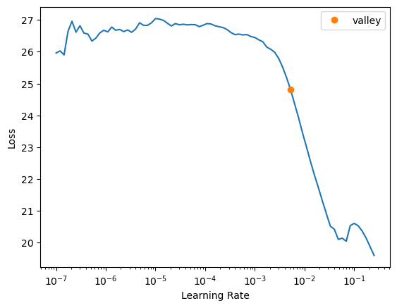
learn.fit(10, lr=0.0001)
| epoch | train_loss | valid_loss | batch_accuracy | time |
|---|---|---|---|---|
| 0 | 22.497177 | 19.988018 | 0.115030 | 00:08 |
| 1 | 14.938927 | 12.020883 | 0.097589 | 00:07 |
| 2 | 9.643848 | 8.343630 | 0.099315 | 00:07 |
| 3 | 7.882081 | 7.430155 | 0.099702 | 00:07 |
| 4 | 7.272729 | 6.995084 | 0.099643 | 00:07 |
| 5 | 6.875529 | 6.635660 | 0.099613 | 00:07 |
| 6 | 6.536114 | 6.316277 | 0.099643 | 00:07 |
| 7 | 6.235651 | 6.033361 | 0.099613 | 00:07 |
| 8 | 5.971189 | 5.785527 | 0.099583 | 00:07 |
| 9 | 5.741306 | 5.571390 | 0.099583 | 00:07 |
Once again a very disappointing result. One thing I did learn in this whole process is that doing everything manually, when it comes to machine learning and deep learning, is VERY fiddly and cumbersome. It certainly is a lot to keep track of at this lower level of code.
With that in mind, we should move on to giving this one last go, but instead of a a linear function lets use convolutions, we’ll use some of fastai’s handy tools to help us do this.
Conv2d
We are going to use the nn.Conv2d convolutional method provided by PyTorch. Along with that we will use Pytorch’s F.cross_entropy as the loss function and, as in our simple_net above, we’ll use SGD as our optimiser.
Let’s reprocess our data so that it is ready for this new type of model we are using. Note that:
- we are now using 28*28 pixel matrices for our images rather than 783 pixel vectors
- because convolutions are done on matrices
- we also add a dimension of 1 as the first dimension (view(1,28,28)) because Conv2d takes in ‘channels’ for each image
- 3d images would have 2 channels, 1 for each colour (RGB).
- since we are only dealing with black and white images (one colour) we will deal with only one channel
pixel_value_columns = train_data_split.iloc[:,1:]
label_value_column = train_data_split.iloc[:,:1]

pixel_value_columns = pixel_value_columns.apply(lambda x: x/255)

pixel_value_columns_tensor = torch.tensor(train_data.iloc[:,1:].values).float()
# here we change from image vectors to image matrices and put it in our one channel
pixel_value_matrices_tensor = [row.view(1,28,28) for row in pixel_value_columns_tensor]

label_value_column_tensor = torch.tensor(train_data.iloc[:,:1].values).float()

# F.cross_entropy requires that the labels are tensor of scalar. label values cannot be `FloatTensor` if they are classes (discrete values), must be cast to `LongTensor` (`LongTensor` is synonymous with integer)
train_ds = list(zip(pixel_value_matrices_tensor, label_value_column_tensor.squeeze().type(torch.LongTensor)))

train_dl = DataLoader(train_ds, batch_size=256)
pixel_value_columns = valid_data_split.iloc[:,1:]
label_value_column = valid_data_split.iloc[:,:1]

pixel_value_columns = pixel_value_columns.apply(lambda x: x/255)

pixel_value_columns_tensor = torch.tensor(train_data.iloc[:,1:].values).float()
# here we change from image vectors to image matrices and put it in our one channel
pixel_value_matrices_tensor = [row.view(1,28,28) for row in pixel_value_columns_tensor]

label_value_column_tensor = torch.tensor(train_data.iloc[:,:1].values).float()

# F.cross_entropy requires that the labels are tensor of scalar. label values cannot be `FloatTensor` if they are classes (discrete values), must be cast to `LongTensor` (`LongTensor` is synonymous with integer)
valid_ds = list(zip(pixel_value_matrices_tensor, label_value_column_tensor.squeeze().type(torch.LongTensor)))

valid_dl = DataLoader(valid_ds, batch_size=256)
dls = DataLoaders(train_dl,valid_dl)
xb_,yb_ = first(valid_dl)
xb_.shape,yb_[0]
(torch.Size([256, 1, 28, 28]), tensor(1))
So we have a batch size of 256 of single-channel (1) images of size 28*28. So far so good
let’s try out a kernel size of 3.
Note kernels are a key part of convolutions:
- they are a matrix of weights that essentially scans across the whole image and
- for each of it’s positions we take an element-wise multiplication which is:
- the sum
- of each of the products
- of each of it’s weights,
- and each of the the pixels it is covering
- an activation is produced for each kernal position and a new matrix is produced as a result.
Look up Chapter 13 Convolutions in fastai’s fastbook for more information.
ks=3
simple_conv_net = nn.Sequential(
    nn.Conv2d(1,30, kernel_size=3, padding=1),
    nn.ReLU(),
    nn.Conv2d(30,1, kernel_size=3, padding=1)
)
Lets see what shape our output will have with this model.
simple_conv_net(xb_).shape
torch.Size([256, 1, 28, 28])
This is not something we can use to do classification, since we need a single output activation per image, not a 28×28 map of activations. One way to deal with this is to use enough stride-2 convolutions, and padding of 1, such that the final layer is size 10.
Stride is the amount of pixels that the kernel moves by after each position. And the general formula for resultant matrix size is
(n + 2*pad - ks)//stride + 1wherepadis the padding,strideis the stride andksis the kernel size. stride-2 convolutions are useful for decreasing the size of our outputs, and stride-1 convolutions are useful for adding layers without changing the output size
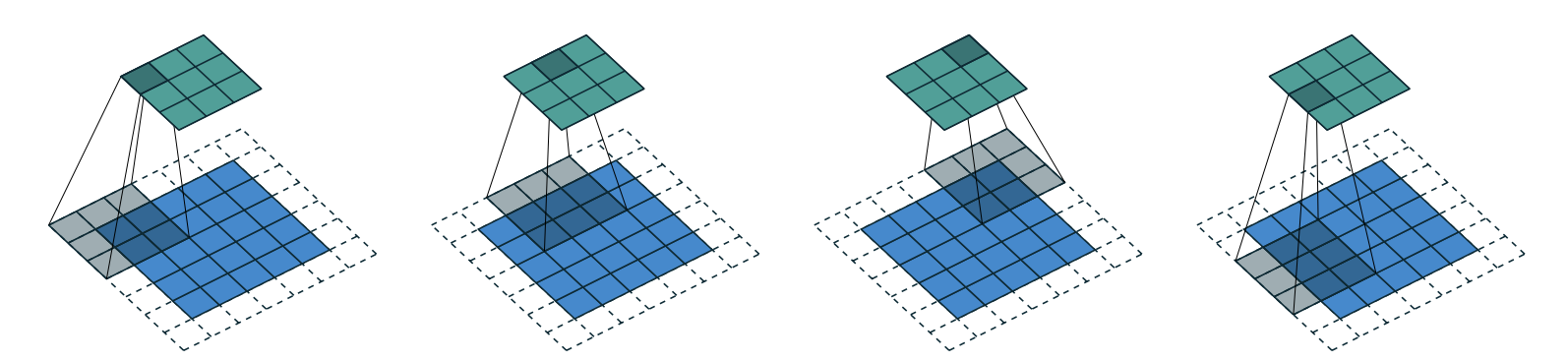
Padding is number of pixels added to the outside of our image. Without padding, and with a stride-1 (no change in output size due to slide) the output matrix will lose size on each dimension. This is due to the fact that the kernel will not go boyond the edges of the image itself. We can counteract this by adding padding. The necessary padding on each side to keep the same shape is
ks//2. (see image below that shows how the image can move further with a padding of 2 added)
The function below is created and used for the sake of easier manipulation of the key factors (input and output channels, stride, etc.)
def conv(ni, nf, ks=3, act=True):
    res = nn.Conv2d(ni, nf, stride=2, kernel_size=ks, padding=ks//2)
    if act: res = nn.Sequential(res, nn.ReLU())
    return res
simple_conv_net = nn.Sequential(
    nn.Conv2d(1,4, stride=2, kernel_size=ks, padding=ks//2),
    nn.ReLU(),
    nn.Conv2d(4,16, stride=2, kernel_size=ks, padding=ks//2),
    nn.ReLU(),
    nn.Conv2d(16,32, stride=2, kernel_size=ks, padding=ks//2),
    nn.ReLU(),
    nn.Conv2d(32,64, stride=2, kernel_size=ks, padding=ks//2),
    nn.ReLU(),
    nn.Conv2d(64,10, stride=2, kernel_size=ks, padding=ks//2),
    Flatten()
)
simple_conv_net(xb_).shape
torch.Size([256, 10])
10 activations/outputs, one for each class (digit), just what we wanted!
Note how the only thing I adapted in the end was the number of layers and the number of channels in and out in each layer.
Now we can give this model a try.
learn = Learner(dls, simple_conv_net, opt_func=SGD,
                loss_func=F.cross_entropy, metrics=accuracy)
learn.lr_find()
SuggestedLRs(valley=0.019054606556892395)
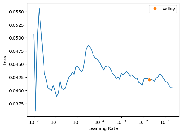
learn.fit(10, lr=0.2)
| epoch | train_loss | valid_loss | accuracy | time |
|---|---|---|---|---|
| 0 | 0.029442 | 0.231421 | 0.944405 | 00:04 |
| 1 | 0.030254 | 0.083334 | 0.973571 | 00:04 |
Not too shabby at all! Much better than all the other attempts…
I clearly still have more to learn here as I still would have expected to gain better results with my Linear Nueral Net (simple_net). Hopefully one day I will figure out where I went wrong or whether I should never have expected any better in the first place!
The final thing left to do is make predictions on the test set using our model and submit the results.
Submitting Results
Lets first format our test data in the same way that we formated our training data, as this is what our model is expecting.
path.ls()
(#3) [Path('../input/digit-recognizer/sample_submission.csv'),Path('../input/digit-recognizer/train.csv'),Path('../input/digit-recognizer/test.csv')]
test_df = pd.read_csv(path/'test.csv')
test_df.describe()
| pixel0 | pixel1 | pixel2 | pixel3 | pixel4 | pixel5 | pixel6 | pixel7 | pixel8 | pixel9 | ... | pixel774 | pixel775 | pixel776 | pixel777 | pixel778 | pixel779 | pixel780 | pixel781 | pixel782 | pixel783 | |
|---|---|---|---|---|---|---|---|---|---|---|---|---|---|---|---|---|---|---|---|---|---|
| count | 28000.0 | 28000.0 | 28000.0 | 28000.0 | 28000.0 | 28000.0 | 28000.0 | 28000.0 | 28000.0 | 28000.0 | ... | 28000.000000 | 28000.000000 | 28000.000000 | 28000.000000 | 28000.000000 | 28000.0 | 28000.0 | 28000.0 | 28000.0 | 28000.0 |
| mean | 0.0 | 0.0 | 0.0 | 0.0 | 0.0 | 0.0 | 0.0 | 0.0 | 0.0 | 0.0 | ... | 0.164607 | 0.073214 | 0.028036 | 0.011250 | 0.006536 | 0.0 | 0.0 | 0.0 | 0.0 | 0.0 |
| std | 0.0 | 0.0 | 0.0 | 0.0 | 0.0 | 0.0 | 0.0 | 0.0 | 0.0 | 0.0 | ... | 5.473293 | 3.616811 | 1.813602 | 1.205211 | 0.807475 | 0.0 | 0.0 | 0.0 | 0.0 | 0.0 |
| min | 0.0 | 0.0 | 0.0 | 0.0 | 0.0 | 0.0 | 0.0 | 0.0 | 0.0 | 0.0 | ... | 0.000000 | 0.000000 | 0.000000 | 0.000000 | 0.000000 | 0.0 | 0.0 | 0.0 | 0.0 | 0.0 |
| 25% | 0.0 | 0.0 | 0.0 | 0.0 | 0.0 | 0.0 | 0.0 | 0.0 | 0.0 | 0.0 | ... | 0.000000 | 0.000000 | 0.000000 | 0.000000 | 0.000000 | 0.0 | 0.0 | 0.0 | 0.0 | 0.0 |
| 50% | 0.0 | 0.0 | 0.0 | 0.0 | 0.0 | 0.0 | 0.0 | 0.0 | 0.0 | 0.0 | ... | 0.000000 | 0.000000 | 0.000000 | 0.000000 | 0.000000 | 0.0 | 0.0 | 0.0 | 0.0 | 0.0 |
| 75% | 0.0 | 0.0 | 0.0 | 0.0 | 0.0 | 0.0 | 0.0 | 0.0 | 0.0 | 0.0 | ... | 0.000000 | 0.000000 | 0.000000 | 0.000000 | 0.000000 | 0.0 | 0.0 | 0.0 | 0.0 | 0.0 |
| max | 0.0 | 0.0 | 0.0 | 0.0 | 0.0 | 0.0 | 0.0 | 0.0 | 0.0 | 0.0 | ... | 253.000000 | 254.000000 | 193.000000 | 187.000000 | 119.000000 | 0.0 | 0.0 | 0.0 | 0.0 | 0.0 |
8 rows × 784 columns
def dataset_from_dataframe(dframe):
    pixel_value_columns = dframe.iloc[:,1:]
    label_value_column = dframe.iloc[:,:1]

    pixel_value_columns = pixel_value_columns.apply(lambda x: x/255)

    pixel_value_columns_tensor = torch.tensor(train_data.iloc[:,1:].values).float()
    pixel_value_matrices_tensor = [row.view(1,28,28) for row in pixel_value_columns_tensor]

    label_value_column_tensor = torch.tensor(train_data.iloc[:,:1].values).float()

    return list(zip(pixel_value_matrices_tensor, label_value_column_tensor.squeeze().type(torch.LongTensor)))
Notice how we didn’t include the final step of creating a dataloader here, like we did for our training and validation data earlier. That’s because, for some reason, we now need to use the test_dl method on the dls object of our learn. I think it is something to do with how I have done this all manaully in a way that we normally wouldn’t in real practice. (for the sake of learning). For example there is the fact that I earlier used DataLoader on the training and validation data instead of ImageDataLoaders or DataBlock with the appropriate input and output types declared (ImageBlock and CategoryBlock respectively).
The methods used below were acquired from this comment in the fastai forums.
test_dset = dataset_from_dataframe(test_df)
test_dl = learn.dls.test_dl(test_dset, num_workers=0, shuffle=False)
test_xb,test_yb = first(test_dl)
test_xb.shape,test_yb.shape
(torch.Size([256, 1, 28, 28]), torch.Size([256]))
Let’s now look at the output of our model
preds = learn.get_preds(dl=test_dl)
preds
(tensor([[ -6.2389,  17.9150,   4.8627,  ...,   2.7307,   1.3093, -10.6259],
         [ 20.6565, -13.0968,   3.0954,  ...,  -3.3692,  -4.1910,   7.7431],
         [-15.5415,  14.7798,  -1.0664,  ...,   0.7134,   2.7963,  -0.1235],
         ...,
         [ 19.4675, -10.6216,   7.1559,  ..., -11.9363,  -3.5295,   1.6469],
         [ -5.9829,   5.2299,  18.4540,  ...,   0.2917,   1.4718, -15.1106],
         [ -8.3286,   2.4987,  33.8273,  ...,   0.8742,   2.4564,  -6.7401]]),
 tensor([1, 0, 1,  ..., 0, 2, 2]))
x,y = preds
x.shape,y.shape
(torch.Size([33600, 10]), torch.Size([33600]))
looks like we are getting tuples as our output. The first item in each tuple is likely to be the activation that corresponds to each possible class that we are classifying our inputs by (each possible digit). The second item in the tuple wuold then be the index of the highest activation in the first item in the tuple. Let’s print a few tuple pairs out to confirm this.
x[0],y[0],x[1],y[1],x[2],y[2],x[-1],y[-1]
(tensor([-6.3086, 16.6723,  3.9996, -3.6847,  3.7977, -6.9672, -1.0412,  0.2652,
          0.1488, -9.8842]),
 tensor(1),
 tensor([ 18.2848, -14.1513,  -0.3664,  -7.7865,  -0.5604,  -2.1511,   2.6904,
           4.7438,  -3.6372,   5.4869]),
 tensor(0),
 tensor([-15.3868,  14.9102,  -2.5896,  -0.6112,  -0.1320,  -0.6092,  -2.6725,
           0.1352,   2.4254,   0.4133]),
 tensor(1),
 tensor([ -7.2539,   1.8877,  29.6757,   7.0085,  -5.6263,  -4.1780, -17.5217,
           1.9317,   2.4628,  -7.4709]),
 tensor(2))
Yep, seems we were right. And since the index of the activations corresponds to the actual values of our classes (0-9) our predictions are directly the values given to us in the second item of each outputted prediction tuple. So let’s get our submission data ready. First, we get a list of our single value predictions, using a list comprehension.
# .numpy() turns the scalar tensors into normal scalar variable in python
predictions_list = [pred.numpy() for pred in y]
pred_labels = pd.Series(predictions_list, name="Label")
pred_labels
0        1
1        0
2        1
3        4
4        0
        ..
33595    6
33596    0
33597    0
33598    2
33599    2
Name: Label, Length: 33600, dtype: object
let’s look at our submission example
ss = pd.read_csv(path/'sample_submission.csv')

ss
| ImageId | Label | |
|---|---|---|
| 0 | 1 | 0 |
| 1 | 2 | 0 |
| 2 | 3 | 0 |
| 3 | 4 | 0 |
| 4 | 5 | 0 |
| ... | ... | ... |
| 27995 | 27996 | 0 |
| 27996 | 27997 | 0 |
| 27997 | 27998 | 0 |
| 27998 | 27999 | 0 |
| 27999 | 28000 | 0 |
28000 rows × 2 columns
Now we simply need to replace the blank labels with our predicted ones (see competition guidlines).
ss['Label'] = pred_labels

ss
| ImageId | Label | |
|---|---|---|
| 0 | 1 | 1 |
| 1 | 2 | 0 |
| 2 | 3 | 1 |
| 3 | 4 | 4 |
| 4 | 5 | 0 |
| ... | ... | ... |
| 27995 | 27996 | 6 |
| 27996 | 27997 | 0 |
| 27997 | 27998 | 8 |
| 27998 | 27999 | 0 |
| 27999 | 28000 | 7 |
28000 rows × 2 columns
Looks good! now we can submit this to kaggle.
We can do it straight from this note book if we are running it on Kaggle, otherwise we can use the API
In this case I did it directly using the kaggle notebook UI and selecting my ‘subm.csv’ file from the output folder there (see these guidelines)
# this outputs the actual file
ss.to_csv('subm.csv', index=False)
#this shows the head (first few lines)
!head subm.csv
ImageId,Label
1,1
2,0
3,1
4,4
5,0
6,0
7,7
8,3
9,5
After submitting the results, a score of 0.10217 (just above the bottom 10th percentile on the leaderboard - top being 1.0000). This is incredibly disappointing considering that 0.80750 was given for my previous model which wasn’t even deep learning.
Taking a guess, I think perhaps we overfit on the training data, the accuracy was super high but I can also see that it did get to a point where it went down after going up, and then up again. My understanding as that this is also signs of overfitting.
Second attempt using 1cycle instead
Instead of using a static learning rate, we can actually have it be dynamic over the course of the epoch:
- start with low learning rate, since we don’t want the model to instantly diverge
- end with low learning rate also, since we don’t want to jump over our point of minimum
- ramp the learning rate up, and then back down, in between the start and end.
By training with higher learning rates (in between start and end), we:
- train faster — a phenomenon named super-convergence.
- we overfit less because we skip over the sharp local minima to end up in a smoother (and therefore more generalizable) part of the loss.
This type of training is called 1cycle training and we can do it via the fit_one_cycle method on our Learner object.
let’s reinatiate our learn.
new_learn = Learner(dls, simple_conv_net, opt_func=SGD,
                loss_func=F.cross_entropy, metrics=accuracy)
Now let’s try fit_one_cycle over 1 epoch.
new_learn.fit_one_cycle(1)
| epoch | train_loss | valid_loss | accuracy | time |
|---|---|---|---|---|
| 0 | 0.030641 | 0.032126 | 0.989554 | 00:05 |
Looks good to me, but so did the attempt where we just used fit so I won’t get excited yet. Let’s sumbit it and see how it goes…
test_dl = new_learn.dls.test_dl(test_dset, num_workers=0, shuffle=False)

preds = new_learn.get_preds(dl=test_dl)
x,y = preds
predictions_list = [pred.numpy() for pred in y]

pred_labels = pd.Series(predictions_list, name="Label")
pred_labels

ss = pd.read_csv(path/'sample_submission.csv')

ss['Label'] = pred_labels

# this outputs the actual file
ss.to_csv('subm.csv', index=False)
#this shows the head (first few lines)
!head subm.csv
ImageId,Label
1,1
2,0
3,1
4,4
5,0
6,0
7,7
8,3
9,5
Seeing the head of the submissin file above and noticing that it was the exact same as the one we got for learn made alarm bells ring. I did some investigating and found that no matter how many times I created a new Learner and re-ran fit or fit_one_cycle, I kept getting the same results. There wasn’t much no point in submitting the results from fit_one_cycle but I did it anyway just for the sake of completeness (got the exact same score of 0.10217 as before, unsurprisingly).
Conclusion
Although no progress was made in terms of model improvement (and therefore getting further on the leader board competition) a lot was learned in terms of neural net architectures. A lot was also learned in how those architectures are put together in PyTorch, although the underwhelming results showed me that a lot about this is yet to be learned!
Before trying to fill in those gaps, i’ll continue in trying to get higher on the competition leaderboard, this time i’ll do it using all the fastai tools I have learned thus far. I’ll do this in a separate notebook..