Gurtaj's blog!

Introduction

This notebook aims to implement a simple two-layer neural network and train it on the MNIST digit recognizer dataset.

I have previously tried this very unsuccessfully and, in attempt to figure out where I went wrong, I stumbled upon this notebook by Samson Zhang which details his steps in creating such a model without any Pytorch or TensorFlow, just numpy (and some pandas and matplotlib).

In this notebook I am going to attempt to recreate his model to enhace my current understanding of the underlying math of neural networks.

# This Python 3 environment comes with many helpful analytics libraries installed
# It is defined by the kaggle/python Docker image: https://github.com/kaggle/docker-python
# For example, here's several helpful packages to load

import numpy as np # linear algebra
import pandas as pd # data processing, CSV file I/O (e.g. pd.read_csv)

# Input data files are available in the read-only "../input/" directory
# For example, running this (by clicking run or pressing Shift+Enter) will list all files under the input directory

import os
for dirname, _, filenames in os.walk('/kaggle/input'):
    for filename in filenames:
        print(os.path.join(dirname, filename))

# You can write up to 20GB to the current directory (/kaggle/working/) that gets preserved as output when you create a version using "Save & Run All" 
# You can also write temporary files to /kaggle/temp/, but they won't be saved outside of the current session

/kaggle/input/digit-recognizer/sample_submission.csv
/kaggle/input/digit-recognizer/train.csv
/kaggle/input/digit-recognizer/test.csv

from matplotlib import pyplot as plt

First we get the MNIST train data into a pandas dataframe (see list of filepaths printed after first cell in this notebook).

# %who
data = pd.read_csv('/kaggle/input/digit-recognizer/train.csv')

let’s look at it.

data

	label	pixel0	pixel1	pixel2	pixel3	pixel4	pixel5	pixel6	pixel7	pixel8	...	pixel774	pixel775	pixel776	pixel777	pixel778	pixel779	pixel780	pixel781	pixel782	pixel783
0	1	0	0	0	0	0	0	0	0	0	...	0	0	0	0	0	0	0	0	0	0
1	0	0	0	0	0	0	0	0	0	0	...	0	0	0	0	0	0	0	0	0	0
2	1	0	0	0	0	0	0	0	0	0	...	0	0	0	0	0	0	0	0	0	0
3	4	0	0	0	0	0	0	0	0	0	...	0	0	0	0	0	0	0	0	0	0
4	0	0	0	0	0	0	0	0	0	0	...	0	0	0	0	0	0	0	0	0	0
...	...	...	...	...	...	...	...	...	...	...	...	...	...	...	...	...	...	...	...	...	...
41995	0	0	0	0	0	0	0	0	0	0	...	0	0	0	0	0	0	0	0	0	0
41996	1	0	0	0	0	0	0	0	0	0	...	0	0	0	0	0	0	0	0	0	0
41997	7	0	0	0	0	0	0	0	0	0	...	0	0	0	0	0	0	0	0	0	0
41998	6	0	0	0	0	0	0	0	0	0	...	0	0	0	0	0	0	0	0	0	0
41999	9	0	0	0	0	0	0	0	0	0	...	0	0	0	0	0	0	0	0	0	0

42000 rows × 785 columns

We can see that:

each row is an image
the first column of each row is the label of the image
every column besides the first fow is the value of a particular pixel in that image.

Each pixel has a value between 0 and 255 (0 being completely off and 255 being completely on). See the competition dataset description for more details.

# Load the data into a numpy array
data = np.array(data)

# right now the data shape is (42_000, 785) we transpose this to (785, 42_000)
# that will be split to Y: (1, 42_000) and X: (784, 42_000)
# this is because our first set of weights, that we multiply the inputs by, are going to be (10, 784)
# and for matrix multipication the number of columns in the first matrix (the weights) must be equal to the number of rows in the second (the input, X)
data_transposed = data.T

# Get the number of rows and columns in the data
n_rows, n_columns = data_transposed.shape

# Shuffle the data before splitting into validation and training sets
# This helps to prevent the dev and training sets from being biased
np.random.shuffle(data)

# Split the data into the validation and training sets
data_valid = data_transposed[:,0:1000]
# get first row for image labels
Y_valid = data_valid[0]
# get the rest of the rows for image pixel values
X_valid = data_valid[1:n_rows]
# squash pixel values to values between 0 and 1
X_valid = X_valid / 255.

data_train = data_transposed[:,1000:n_columns]
Y_train = data_train[0]
X_train = data_train[1:n_rows]
X_train = X_train / 255.

# Get the number of rows in the training set
_, m_train = X_train.shape

# Print the shapes of the validation and training sets
print(f"Shape of validation set: {data_valid.shape}",)
print(f"Shape of training set: {data_train.shape}")

Shape of validation set: (785, 1000)
Shape of training set: (785, 41000)

Now we have 1000 samples in our validation set and 41000 samples in our training set.

Out Neural Network will have a simple 2-layer architecture.

input layer will have 784 units corresponding to the 784 pixels in each 28x28 image.
hidden layer will have 10 units, with ReLU activation.
output layer will have 10 units corresponding to the ten digit classes, with softmax activation.

Forward propogation

unactivated first layer values, $Z^{[1]}$:
$Z^{[1]} = W^{[1]} X + b^{[1]}$
first layer activation values, $A^{[1]}$:
$A^{[1]} = g_{\text{ReLU}}(Z^{[1]})$
unactivated second layer values, $Z^{[2]}$:
$Z^{[2]} = W^{[2]} A^{[1]} + b^{[2]}$
second layer activation values, $A^{[2]}$:
$A^{[2]} = g_{\text{softmax}}(Z^{[2]})$

$X$: 784 inputs x columns/samples.
$W^{[1]}$ 10 matrices of 784 weights.
$b^{[1]}$ an array of 10 biases.
$Z^{[1]}$: 10 measurements x rows/samples.
$A^{[1]}$: 10 activations x rows/samples.
$W^{[2]}$ 10 matrices of 10 weights.
$b^{[2]}$ an array of 10 biases.
$Z^{[2]}$: 10 measurements x rows/samples.
$A^{[2]}$: 10 activations x rows/samples.

Backward propogation

second layer
- difference between output, $A^{[2]}$, and ground truth, $Y$ (the loss function):
  $dZ^{[2]} = A^{[2]} - Y$
- how much $W^{[2]}$ contributed to the above difference/error (the derivative of the loss function wrt $W^{[2]}$):
  $dW^{[2]} = \frac{1}{m} dZ^{[2]} A^{[1]T}$
- how much $b^{[2]}$ contributed to the above difference/error (the derivative of the loss function wrt $b^{[2]}$):
  $dB^{[2]} = \frac{1}{m} \Sigma {dZ^{[2]}}$
first layer/hidden layer
- now we determine how much the hidden layer/first layer contributed towards the error. $W^{[2]T} dZ^{[2]}$ is applying the weights, in reverse (transposed), to the errors of the second layer, in order to get to the errors of the first layer. $g^{[1]\prime}$ is the derivative of the activation function, which we also need in order to get the propper error for the first layer.:
  $W^{[2]T} dZ^{[2]} .* g^{[1]\prime} (Z^{[1]})$
- how much $W^{[1]}$ contributed to the above difference/error (the derivative of the loss function wrt $W^{[1]}$):
  $dW^{[1]} = \frac{1}{m} dZ^{[1]} A^{[0]T}$
- how much $b^{[1]}$ contributed to the above difference/error (the derivative of the loss function wrt $b^{[1]}$):
  $dB^{[1]} = \frac{1}{m} \Sigma {dZ^{[1]}}$

$Y$: 10 x rows/samples (one hot encoded array of 10 values for each row/sample - only one 1 value in each array, the rest are 0. The 1 corresponding to the index of the correct digit label)
$dZ^{[2]}$: 10 errors x rows/samples.
$dW^{[2]}$: 10 gradients x 10 weights.
$db^{[2]}$: 10 gradients x 10 biases.
$dZ^{[1]}$: 10 errors x rows/samples.
$dW^{[1]}$: 784 gradients x 10 weights matrices.
$db^{[1]}$: 1 gradients x 10 biases.

NOTE the $^T$ notation for transposed ($A^{[1]T}$ is just $A^{[1]}$ transposed)

Parameter updates

$W^{[2]} := W^{[2]} - \alpha dW^{[2]}$
$b^{[2]} := b^{[2]} - \alpha db^{[2]}$
$W^{[1]} := W^{[1]} - \alpha dW^{[1]}$
$b^{[1]} := b^{[1]} - \alpha db^{[1]}$

$\alpha$: learning rate - a hyperparameter picked by us.

# init params with uniformly distributed values in the range -0.5 to 0.5
def init_params():
    W1 = np.random.rand(10, 784) - 0.5
    b1 = np.random.rand(10, 1) - 0.5
    W2 = np.random.rand(10, 10) - 0.5
    b2 = np.random.rand(10, 1) - 0.5
    return W1, b1, W2, b2

# returns input directly if it is positive, or 0 if input is negative
# np.maximum compares it's two input values and returns whichever is higher
def ReLU(Z):
    return np.maximum(Z, 0)

# note this is not the 'numerically stable' version of softmax
# this is fine since we won't be taking the exponent of any particularly large numbers here
def softmax(Z):
    each_individual_exponent = np.exp(Z)
    sum_over_all_exponents = sum(each_individual_exponent)
    activations = each_individual_exponent / sum_over_all_exponents
    return activations

def forward_propagation(W1, b1, W2, b2, X):
    # from .dot docstring: If both a and b are 2-D arrays, it is matrix multiplication, but using matmul or a @ b is preferred.
    Z1 = W1.dot(X) + b1
    A1 = ReLU(Z1)
    Z2 = W2.dot(A1) + b2
    A2 = softmax(Z2)
    return Z1, A1, Z2, A2

# this is the derivative of the ReLU function, it is 1 for all values above 0 and 0 for all values below it below it.
# since the positive part of the ReLU function is a linear function (returns input directly), the gradient is 1
# since the negative part of the ReLU function is just 0, the gradient is also 0
# and when booleans are converted to numbers `True` is always `1` and `False` is always `0` 
def ReLU_deriv(Z):
    return Z > 0

def one_hot(Y):
    """
    Convert the labels into one-hot encoded vectors.
    """
    # note that number of columns in `Y` is 1; 1 digit for each label
    n_rows = Y.size
    
    # Create a one-hot encoded vector for each label
    # np.zeros creates array/matrix of all zeros of the requested size
    # so the dimensions here are going to be (784 samples, 1 label array for each, 10 values in each 1-hot encoded label array; 1 for each digit)
    one_hot_Y = np.zeros((n_rows, Y.max() + 1))
    # go through each of the rows of one_hot_Y, from start to end, and for every corresponding column denoted by Y, set it to `1`
    one_hot_Y[np.arange(len(one_hot_Y)), Y] = 1
    
    # right now the shape of `one_hot_Y` is (n_rows, 10), we need to transpose this to (10, n_rows)
    # this is because A2 is going to be of shape (10, n_rows) and we will be subtracting one_hot_y from A2 so their sizes must match
    one_hot_Y = one_hot_Y.T
    
    return one_hot_Y

def backward_propagation(Z1, A1, Z2, A2, W1, W2, X, Y):
    n_rows = Y.size
    one_hot_Y = one_hot(Y)
    dZ2 = A2 - one_hot_Y
    # in order to matrix multiply dZ2 (10, n_columns) by A1, we transpose A1 from (10, n_columns) to (n_columns, 10) 
    dW2 = 1 / n_rows * dZ2.dot(A1.T)
    db2 = 1 / n_rows * np.sum(dZ2)
    # although it's mathematically valied to multiply W2 (10, 10) by dZ2 (10, n_col)
    # we transpose W2 so that the weights are applied in the right order (kind of the reverse of how they are applied in forward propagation)
    dZ1 = W2.T.dot(dZ2) * ReLU_deriv(Z1)
    # in order to multiply `dZ1` (10, n_columns) by `X` (784, n_columns) we transpose it to (n_columns, 784) 
    dW1 = 1 / n_rows * dZ1.dot(X.T)
    db1 = 1 / n_rows * np.sum(dZ1)
    return dW1, db1, dW2, db2

def update_params(W1, b1, W2, b2, dW1, db1, dW2, db2, lr):
    W1 = W1 - lr * dW1
    b1 = b1 - lr * db1    
    W2 = W2 - lr * dW2  
    b2 = b2 - lr * db2    
    return W1, b1, W2, b2

ASIDE

The softmax function

Here I am just, for my own understanding, testing how the softmax function works.

test_measurements = [0,1,2,3]

print(f"exponent for each element in array:{np.exp(test_measurements[0]),np.exp(test_measurements[1]),np.exp(test_measurements[2]),np.exp(test_measurements[3])}",
      f"exponent over whole array: {np.exp(test_measurements)}",
      f"sum of each indidual element's exponent vs sum over exponent over whole array: {np.exp(test_measurements[0])+np.exp(test_measurements[1])+np.exp(test_measurements[2])+np.exp(test_measurements[3]),sum(np.exp(test_measurements))}",
      f"each individal element's exponent divided by sum over exponent over whole array: {np.exp(test_measurements[0])/sum(np.exp(test_measurements)),np.exp(test_measurements[1])/sum(np.exp(test_measurements)),np.exp(test_measurements[2])/sum(np.exp(test_measurements)),np.exp(test_measurements[3])/sum(np.exp(test_measurements))}",
      f"exponent over whole array divided by sum over exponent over whole array: {np.exp(test_measurements)/sum(np.exp(test_measurements))}",
      sep='\n\n'
     )

exponent for each element in array:(1.0, 2.718281828459045, 7.38905609893065, 20.085536923187668)

exponent over whole array: [ 1.          2.71828183  7.3890561  20.08553692]

sum of each indidual element's exponent vs sum over exponent over whole array: (31.19287485057736, 31.19287485057736)

each individal element's exponent divided by sum over exponent over whole array: (0.03205860328008499, 0.08714431874203257, 0.23688281808991016, 0.6439142598879724)

exponent over whole array divided by sum over exponent over whole array: [0.0320586  0.08714432 0.23688282 0.64391426]

I can see now that all is fine. I was thinking that it’s possible it could combine each individual value of np.exp(Z)/sum(np.exp(Z)), (one for each item inZ and therefore in np.exp(Z)) and not return them separately. I see now that this is not the case.

The `one_hot` function

I understand the concept of one-hot encoding fine. I just want to play around with the actual trainind data labels to see if what is going on in one_hot is in fact correct

one_hot_Y = np.zeros((Y_train.size, Y_train.max() + 1))

one_hot_Y,len(one_hot_Y),Y_train.size,Y_train.max()

(array([[0., 0., 0., ..., 0., 0., 0.],
        [0., 0., 0., ..., 0., 0., 0.],
        [0., 0., 0., ..., 0., 0., 0.],
        ...,
        [0., 0., 0., ..., 0., 0., 0.],
        [0., 0., 0., ..., 0., 0., 0.],
        [0., 0., 0., ..., 0., 0., 0.]]),
 41000,
 41000,
 9)

So above we see that we have created a matrix of matrix of 41000 arrays, each of 10 0 values

# array of integers going from 0 upto, but not including, Y_train.size (41,000)
np.arange(len(one_hot_Y))

array([    0,     1,     2, ..., 40997, 40998, 40999])

Here, using np.arange we have created an array of integers going from index 0 upto, but not including, index Y_train.size (41,000)

# go through each of the 41,000 rows of one_hot_Y, and for every corresponding column denoted by Y_train, set it to `1`
# so basically `np.arange(len(one_hot_Y))` is an array of all the x coordinates that we are setting to 1
# and Y_train is an array of all the y coordinates that we are setting to 1
one_hot_Y[np.arange(len(one_hot_Y)), Y_train] = 1

So now we are accessing one_hot_Y via two arrays:

np.arange(len(one_hot_Y)) is an array of all the x coordinates
Y_train is an array of all the y coordinates (remember it is just an array of 41000 values which range from 0-9 - these correspond to each possible digit, and also, conveniently, to each possible index in the 41,000 arrays in one_hot_Y

Each position in one_hot_Y that is specified by these (x,y) coordinates is therefore set to 1. Let’s see how one_hot_Y looks now.

one_hot_Y,one_hot_Y.shape,one_hot_Y.T.shape

(array([[0., 0., 0., ..., 1., 0., 0.],
        [1., 0., 0., ..., 0., 0., 0.],
        [0., 0., 0., ..., 0., 0., 1.],
        ...,
        [0., 0., 0., ..., 1., 0., 0.],
        [0., 0., 0., ..., 1., 0., 0.],
        [0., 0., 1., ..., 0., 0., 0.]]),
 (41000, 10),
 (10, 41000))

No longer is it all 0s!

Let’s play around with a smaller example than Y_train just to confirm that this is exactly what is going on.

numpy_array = np.array([[1,2,3],[3,2,1]])

numpy_array

array([[1, 2, 3],
       [3, 2, 1]])

reference_numpy_array_x = np.array([1,0])
reference_numpy_array_y = np.array([2,0])

numpy_array[reference_numpy_array_x,reference_numpy_array_y] = 6
numpy_array

array([[6, 2, 3],
       [3, 2, 6]])

Great. I’m now confident that I understand what is going on in one_hot. I hope this makes it clearer for anyone reading also…

END ASIDE

Let’s continue with the rest of our functions.

def get_predictions(A2):
    """
    Get predicted label/class.
    """
    # this returns the index of highest activation in each array.
    # the index is also, conveniently, the same as the label value that we want to predict (0-9)
    return np.argmax(A2, 0)

def get_accuracy(predictions, Y):
    print(predictions, Y)
    # return mean accuracy
    # np.sum(predictions == Y) is a sum of all the `1`s (corrects precitions) and `0`s (incorrect predictions)
    # predictions.size is the total number of prections (also equal to Y.size)
    return np.sum(predictions == Y) / predictions.size

# iterations is the number of times we want to run our training loop
def gradient_descent(X, Y, lr, iterations):
    W1, b1, W2, b2 = init_params()
    for i in range(iterations):
        Z1, A1, Z2, A2 = forward_propagation(W1, b1, W2, b2, X)
        dW1, db1, dW2, db2 = backward_propagation(Z1, A1, Z2, A2, W1, W2, X, Y)
        W1, b1, W2, b2 = update_params(W1, b1, W2, b2, dW1, db1, dW2, db2, lr)
        # the below is executed on every 10th iteration (i % 10 == 0)
        if i % 10 == 0:
            print("Iteration: ", i)
            predictions = get_predictions(A2)
            print(get_accuracy(predictions, Y))
    return W1, b1, W2, b2

ASIDE

The below snippet is just me figuring out which index is returned by np.argmax depending on which dimension we choose.

test_array = np.array([[0,2,8,0,1,3], # index of highest value along this dimension = 2
                       [0,2,2,8,1,5]])# index of highest value along this dimension = 3
# highest index in dm:  0,0,0,1,0,1

np.argmax(test_array,1),np.argmax(test_array,0)

(array([2, 3]), array([0, 0, 0, 1, 0, 1]))

END ASIDE

Now lets run gradient_descent and see what happens.

W1, b1, W2, b2 = gradient_descent(X_train, Y_train, 0.1, 500)

784 784 41000 10 1
Iteration:  0
[3 3 9 ... 3 9 3] [7 0 9 ... 7 7 2]
14434146341463414
784 784 41000 10 1
784 784 41000 10 1
784 784 41000 10 1
784 784 41000 10 1
784 784 41000 10 1
784 784 41000 10 1
784 784 41000 10 1
784 784 41000 10 1
784 784 41000 10 1
784 784 41000 10 1
Iteration:  10
[3 0 8 ... 3 8 4] [7 0 9 ... 7 7 2]
2752439024390244
784 784 41000 10 1
784 784 41000 10 1
784 784 41000 10 1
784 784 41000 10 1
784 784 41000 10 1
784 784 41000 10 1
784 784 41000 10 1
784 784 41000 10 1
784 784 41000 10 1
784 784 41000 10 1
Iteration:  20
[2 0 9 ... 7 8 4] [7 0 9 ... 7 7 2]
34648780487804876
784 784 41000 10 1
784 784 41000 10 1
784 784 41000 10 1
784 784 41000 10 1
784 784 41000 10 1
784 784 41000 10 1
784 784 41000 10 1
784 784 41000 10 1
784 784 41000 10 1
784 784 41000 10 1
Iteration:  30
[2 0 9 ... 7 9 6] [7 0 9 ... 7 7 2]
41560975609756096
784 784 41000 10 1
784 784 41000 10 1
784 784 41000 10 1
784 784 41000 10 1
784 784 41000 10 1
784 784 41000 10 1
784 784 41000 10 1
784 784 41000 10 1
784 784 41000 10 1
784 784 41000 10 1
Iteration:  40
[9 0 9 ... 7 9 6] [7 0 9 ... 7 7 2]
48236585365853657
784 784 41000 10 1
784 784 41000 10 1
784 784 41000 10 1
784 784 41000 10 1
784 784 41000 10 1
784 784 41000 10 1
784 784 41000 10 1
784 784 41000 10 1
784 784 41000 10 1
784 784 41000 10 1
Iteration:  50
[9 0 9 ... 7 9 6] [7 0 9 ... 7 7 2]
542609756097561
784 784 41000 10 1
784 784 41000 10 1
784 784 41000 10 1
784 784 41000 10 1
784 784 41000 10 1
784 784 41000 10 1
784 784 41000 10 1
784 784 41000 10 1
784 784 41000 10 1
784 784 41000 10 1
Iteration:  60
[9 0 9 ... 7 9 6] [7 0 9 ... 7 7 2]
5894634146341463
784 784 41000 10 1
784 784 41000 10 1
784 784 41000 10 1
784 784 41000 10 1
784 784 41000 10 1
784 784 41000 10 1
784 784 41000 10 1
784 784 41000 10 1
784 784 41000 10 1
784 784 41000 10 1
Iteration:  70
[9 0 9 ... 7 9 6] [7 0 9 ... 7 7 2]
6247317073170732
784 784 41000 10 1
784 784 41000 10 1
784 784 41000 10 1
784 784 41000 10 1
784 784 41000 10 1
784 784 41000 10 1
784 784 41000 10 1
784 784 41000 10 1
784 784 41000 10 1
784 784 41000 10 1
Iteration:  80
[9 0 9 ... 7 9 6] [7 0 9 ... 7 7 2]
6530731707317073
784 784 41000 10 1
784 784 41000 10 1
784 784 41000 10 1
784 784 41000 10 1
784 784 41000 10 1
784 784 41000 10 1
784 784 41000 10 1
784 784 41000 10 1
784 784 41000 10 1
784 784 41000 10 1
Iteration:  90
[9 0 9 ... 7 9 6] [7 0 9 ... 7 7 2]
676609756097561
784 784 41000 10 1
784 784 41000 10 1
784 784 41000 10 1
784 784 41000 10 1
784 784 41000 10 1
784 784 41000 10 1
784 784 41000 10 1
784 784 41000 10 1
784 784 41000 10 1
784 784 41000 10 1
Iteration:  100
[9 0 9 ... 7 9 6] [7 0 9 ... 7 7 2]
6948780487804878
784 784 41000 10 1
784 784 41000 10 1
784 784 41000 10 1
784 784 41000 10 1
784 784 41000 10 1
784 784 41000 10 1
784 784 41000 10 1
784 784 41000 10 1
784 784 41000 10 1
784 784 41000 10 1
Iteration:  110
[0 0 9 ... 7 9 6] [7 0 9 ... 7 7 2]
7111219512195122
784 784 41000 10 1
784 784 41000 10 1
784 784 41000 10 1
784 784 41000 10 1
784 784 41000 10 1
784 784 41000 10 1
784 784 41000 10 1
784 784 41000 10 1
784 784 41000 10 1
784 784 41000 10 1
Iteration:  120
[0 0 9 ... 7 7 6] [7 0 9 ... 7 7 2]
7239512195121951
784 784 41000 10 1
784 784 41000 10 1
784 784 41000 10 1
784 784 41000 10 1
784 784 41000 10 1
784 784 41000 10 1
784 784 41000 10 1
784 784 41000 10 1
784 784 41000 10 1
784 784 41000 10 1
Iteration:  130
[0 0 9 ... 7 7 6] [7 0 9 ... 7 7 2]
7358048780487805
784 784 41000 10 1
784 784 41000 10 1
784 784 41000 10 1
784 784 41000 10 1
784 784 41000 10 1
784 784 41000 10 1
784 784 41000 10 1
784 784 41000 10 1
784 784 41000 10 1
784 784 41000 10 1
Iteration:  140
[0 0 9 ... 7 7 6] [7 0 9 ... 7 7 2]
7462682926829268
784 784 41000 10 1
784 784 41000 10 1
784 784 41000 10 1
784 784 41000 10 1
784 784 41000 10 1
784 784 41000 10 1
784 784 41000 10 1
784 784 41000 10 1
784 784 41000 10 1
784 784 41000 10 1
Iteration:  150
[0 0 9 ... 7 7 6] [7 0 9 ... 7 7 2]
7558292682926829
784 784 41000 10 1
784 784 41000 10 1
784 784 41000 10 1
784 784 41000 10 1
784 784 41000 10 1
784 784 41000 10 1
784 784 41000 10 1
784 784 41000 10 1
784 784 41000 10 1
784 784 41000 10 1
Iteration:  160
[0 0 9 ... 7 7 6] [7 0 9 ... 7 7 2]
7632439024390244
784 784 41000 10 1
784 784 41000 10 1
784 784 41000 10 1
784 784 41000 10 1
784 784 41000 10 1
784 784 41000 10 1
784 784 41000 10 1
784 784 41000 10 1
784 784 41000 10 1
784 784 41000 10 1
Iteration:  170
[0 0 9 ... 7 7 6] [7 0 9 ... 7 7 2]
7710487804878049
784 784 41000 10 1
784 784 41000 10 1
784 784 41000 10 1
784 784 41000 10 1
784 784 41000 10 1
784 784 41000 10 1
784 784 41000 10 1
784 784 41000 10 1
784 784 41000 10 1
784 784 41000 10 1
Iteration:  180
[0 0 9 ... 7 7 6] [7 0 9 ... 7 7 2]
7777073170731708
784 784 41000 10 1
784 784 41000 10 1
784 784 41000 10 1
784 784 41000 10 1
784 784 41000 10 1
784 784 41000 10 1
784 784 41000 10 1
784 784 41000 10 1
784 784 41000 10 1
784 784 41000 10 1
Iteration:  190
[0 0 9 ... 7 7 6] [7 0 9 ... 7 7 2]
7837073170731708
784 784 41000 10 1
784 784 41000 10 1
784 784 41000 10 1
784 784 41000 10 1
784 784 41000 10 1
784 784 41000 10 1
784 784 41000 10 1
784 784 41000 10 1
784 784 41000 10 1
784 784 41000 10 1
Iteration:  200
[0 0 9 ... 7 7 6] [7 0 9 ... 7 7 2]
7890487804878049
784 784 41000 10 1
784 784 41000 10 1
784 784 41000 10 1
784 784 41000 10 1
784 784 41000 10 1
784 784 41000 10 1
784 784 41000 10 1
784 784 41000 10 1
784 784 41000 10 1
784 784 41000 10 1
Iteration:  210
[0 0 9 ... 7 7 6] [7 0 9 ... 7 7 2]
7937073170731708
784 784 41000 10 1
784 784 41000 10 1
784 784 41000 10 1
784 784 41000 10 1
784 784 41000 10 1
784 784 41000 10 1
784 784 41000 10 1
784 784 41000 10 1
784 784 41000 10 1
784 784 41000 10 1
Iteration:  220
[0 0 9 ... 7 7 6] [7 0 9 ... 7 7 2]
7979512195121952
784 784 41000 10 1
784 784 41000 10 1
784 784 41000 10 1
784 784 41000 10 1
784 784 41000 10 1
784 784 41000 10 1
784 784 41000 10 1
784 784 41000 10 1
784 784 41000 10 1
784 784 41000 10 1
Iteration:  230
[0 0 9 ... 7 7 6] [7 0 9 ... 7 7 2]
8016829268292683
784 784 41000 10 1
784 784 41000 10 1
784 784 41000 10 1
784 784 41000 10 1
784 784 41000 10 1
784 784 41000 10 1
784 784 41000 10 1
784 784 41000 10 1
784 784 41000 10 1
784 784 41000 10 1
Iteration:  240
[0 0 9 ... 7 7 6] [7 0 9 ... 7 7 2]
8054146341463415
784 784 41000 10 1
784 784 41000 10 1
784 784 41000 10 1
784 784 41000 10 1
784 784 41000 10 1
784 784 41000 10 1
784 784 41000 10 1
784 784 41000 10 1
784 784 41000 10 1
784 784 41000 10 1
Iteration:  250
[0 0 9 ... 7 7 6] [7 0 9 ... 7 7 2]
8093902439024391
784 784 41000 10 1
784 784 41000 10 1
784 784 41000 10 1
784 784 41000 10 1
784 784 41000 10 1
784 784 41000 10 1
784 784 41000 10 1
784 784 41000 10 1
784 784 41000 10 1
784 784 41000 10 1
Iteration:  260
[0 0 9 ... 7 7 6] [7 0 9 ... 7 7 2]
8129024390243902
784 784 41000 10 1
784 784 41000 10 1
784 784 41000 10 1
784 784 41000 10 1
784 784 41000 10 1
784 784 41000 10 1
784 784 41000 10 1
784 784 41000 10 1
784 784 41000 10 1
784 784 41000 10 1
Iteration:  270
[0 0 9 ... 7 7 6] [7 0 9 ... 7 7 2]
8161219512195121
784 784 41000 10 1
784 784 41000 10 1
784 784 41000 10 1
784 784 41000 10 1
784 784 41000 10 1
784 784 41000 10 1
784 784 41000 10 1
784 784 41000 10 1
784 784 41000 10 1
784 784 41000 10 1
Iteration:  280
[0 0 9 ... 7 7 6] [7 0 9 ... 7 7 2]
8190487804878048
784 784 41000 10 1
784 784 41000 10 1
784 784 41000 10 1
784 784 41000 10 1
784 784 41000 10 1
784 784 41000 10 1
784 784 41000 10 1
784 784 41000 10 1
784 784 41000 10 1
784 784 41000 10 1
Iteration:  290
[0 0 9 ... 7 7 6] [7 0 9 ... 7 7 2]
8216097560975609
784 784 41000 10 1
784 784 41000 10 1
784 784 41000 10 1
784 784 41000 10 1
784 784 41000 10 1
784 784 41000 10 1
784 784 41000 10 1
784 784 41000 10 1
784 784 41000 10 1
784 784 41000 10 1
Iteration:  300
[0 0 9 ... 7 7 6] [7 0 9 ... 7 7 2]
8241219512195121
784 784 41000 10 1
784 784 41000 10 1
784 784 41000 10 1
784 784 41000 10 1
784 784 41000 10 1
784 784 41000 10 1
784 784 41000 10 1
784 784 41000 10 1
784 784 41000 10 1
784 784 41000 10 1
Iteration:  310
[0 0 9 ... 7 7 6] [7 0 9 ... 7 7 2]
8264146341463414
784 784 41000 10 1
784 784 41000 10 1
784 784 41000 10 1
784 784 41000 10 1
784 784 41000 10 1
784 784 41000 10 1
784 784 41000 10 1
784 784 41000 10 1
784 784 41000 10 1
784 784 41000 10 1
Iteration:  320
[0 0 9 ... 7 7 6] [7 0 9 ... 7 7 2]
8286829268292683
784 784 41000 10 1
784 784 41000 10 1
784 784 41000 10 1
784 784 41000 10 1
784 784 41000 10 1
784 784 41000 10 1
784 784 41000 10 1
784 784 41000 10 1
784 784 41000 10 1
784 784 41000 10 1
Iteration:  330
[0 0 9 ... 7 7 6] [7 0 9 ... 7 7 2]
8311463414634146
784 784 41000 10 1
784 784 41000 10 1
784 784 41000 10 1
784 784 41000 10 1
784 784 41000 10 1
784 784 41000 10 1
784 784 41000 10 1
784 784 41000 10 1
784 784 41000 10 1
784 784 41000 10 1
Iteration:  340
[0 0 9 ... 7 7 6] [7 0 9 ... 7 7 2]
833390243902439
784 784 41000 10 1
784 784 41000 10 1
784 784 41000 10 1
784 784 41000 10 1
784 784 41000 10 1
784 784 41000 10 1
784 784 41000 10 1
784 784 41000 10 1
784 784 41000 10 1
784 784 41000 10 1
Iteration:  350
[0 0 9 ... 7 7 6] [7 0 9 ... 7 7 2]
8354878048780487
784 784 41000 10 1
784 784 41000 10 1
784 784 41000 10 1
784 784 41000 10 1
784 784 41000 10 1
784 784 41000 10 1
784 784 41000 10 1
784 784 41000 10 1
784 784 41000 10 1
784 784 41000 10 1
Iteration:  360
[0 0 9 ... 7 7 6] [7 0 9 ... 7 7 2]
8374390243902439
784 784 41000 10 1
784 784 41000 10 1
784 784 41000 10 1
784 784 41000 10 1
784 784 41000 10 1
784 784 41000 10 1
784 784 41000 10 1
784 784 41000 10 1
784 784 41000 10 1
784 784 41000 10 1
Iteration:  370
[0 0 9 ... 7 7 6] [7 0 9 ... 7 7 2]
8392195121951219
784 784 41000 10 1
784 784 41000 10 1
784 784 41000 10 1
784 784 41000 10 1
784 784 41000 10 1
784 784 41000 10 1
784 784 41000 10 1
784 784 41000 10 1
784 784 41000 10 1
784 784 41000 10 1
Iteration:  380
[0 0 9 ... 7 7 6] [7 0 9 ... 7 7 2]
8410731707317073
784 784 41000 10 1
784 784 41000 10 1
784 784 41000 10 1
784 784 41000 10 1
784 784 41000 10 1
784 784 41000 10 1
784 784 41000 10 1
784 784 41000 10 1
784 784 41000 10 1
784 784 41000 10 1
Iteration:  390
[0 0 9 ... 7 7 6] [7 0 9 ... 7 7 2]
8429268292682927
784 784 41000 10 1
784 784 41000 10 1
784 784 41000 10 1
784 784 41000 10 1
784 784 41000 10 1
784 784 41000 10 1
784 784 41000 10 1
784 784 41000 10 1
784 784 41000 10 1
784 784 41000 10 1
Iteration:  400
[0 0 9 ... 7 7 6] [7 0 9 ... 7 7 2]
8445121951219512
784 784 41000 10 1
784 784 41000 10 1
784 784 41000 10 1
784 784 41000 10 1
784 784 41000 10 1
784 784 41000 10 1
784 784 41000 10 1
784 784 41000 10 1
784 784 41000 10 1
784 784 41000 10 1
Iteration:  410
[0 0 9 ... 7 7 6] [7 0 9 ... 7 7 2]
8455853658536585
784 784 41000 10 1
784 784 41000 10 1
784 784 41000 10 1
784 784 41000 10 1
784 784 41000 10 1
784 784 41000 10 1
784 784 41000 10 1
784 784 41000 10 1
784 784 41000 10 1
784 784 41000 10 1
Iteration:  420
[0 0 9 ... 7 7 6] [7 0 9 ... 7 7 2]
8470243902439024
784 784 41000 10 1
784 784 41000 10 1
784 784 41000 10 1
784 784 41000 10 1
784 784 41000 10 1
784 784 41000 10 1
784 784 41000 10 1
784 784 41000 10 1
784 784 41000 10 1
784 784 41000 10 1
Iteration:  430
[0 0 9 ... 7 7 6] [7 0 9 ... 7 7 2]
8480975609756097
784 784 41000 10 1
784 784 41000 10 1
784 784 41000 10 1
784 784 41000 10 1
784 784 41000 10 1
784 784 41000 10 1
784 784 41000 10 1
784 784 41000 10 1
784 784 41000 10 1
784 784 41000 10 1
Iteration:  440
[0 0 9 ... 7 7 6] [7 0 9 ... 7 7 2]
8494146341463414
784 784 41000 10 1
784 784 41000 10 1
784 784 41000 10 1
784 784 41000 10 1
784 784 41000 10 1
784 784 41000 10 1
784 784 41000 10 1
784 784 41000 10 1
784 784 41000 10 1
784 784 41000 10 1
Iteration:  450
[0 0 9 ... 7 7 6] [7 0 9 ... 7 7 2]
850780487804878
784 784 41000 10 1
784 784 41000 10 1
784 784 41000 10 1
784 784 41000 10 1
784 784 41000 10 1
784 784 41000 10 1
784 784 41000 10 1
784 784 41000 10 1
784 784 41000 10 1
784 784 41000 10 1
Iteration:  460
[0 0 9 ... 7 7 6] [7 0 9 ... 7 7 2]
852
784 784 41000 10 1
784 784 41000 10 1
784 784 41000 10 1
784 784 41000 10 1
784 784 41000 10 1
784 784 41000 10 1
784 784 41000 10 1
784 784 41000 10 1
784 784 41000 10 1
784 784 41000 10 1
Iteration:  470
[0 0 9 ... 7 7 6] [7 0 9 ... 7 7 2]
853390243902439
784 784 41000 10 1
784 784 41000 10 1
784 784 41000 10 1
784 784 41000 10 1
784 784 41000 10 1
784 784 41000 10 1
784 784 41000 10 1
784 784 41000 10 1
784 784 41000 10 1
784 784 41000 10 1
Iteration:  480
[0 0 9 ... 7 7 6] [7 0 9 ... 7 7 2]
8546341463414634
784 784 41000 10 1
784 784 41000 10 1
784 784 41000 10 1
784 784 41000 10 1
784 784 41000 10 1
784 784 41000 10 1
784 784 41000 10 1
784 784 41000 10 1
784 784 41000 10 1
784 784 41000 10 1
Iteration:  490
[0 0 9 ... 7 7 6] [7 0 9 ... 7 7 2]
8554146341463414
784 784 41000 10 1
784 784 41000 10 1
784 784 41000 10 1
784 784 41000 10 1
784 784 41000 10 1
784 784 41000 10 1
784 784 41000 10 1
784 784 41000 10 1
784 784 41000 10 1

So that’s about ~84% accuracy on the training data.

Now, let’s create a function for just getting predictions directly, make_predictions, we will pass our inputs and learned weights to this.
And let’s create another function one for viewing individual predictions, test_prediction.

def make_predictions(X, W1, b1, W2, b2):
    _, _, _, A2 = forward_propagation(W1, b1, W2, b2, X)
    predictions = get_predictions(A2)
    return predictions

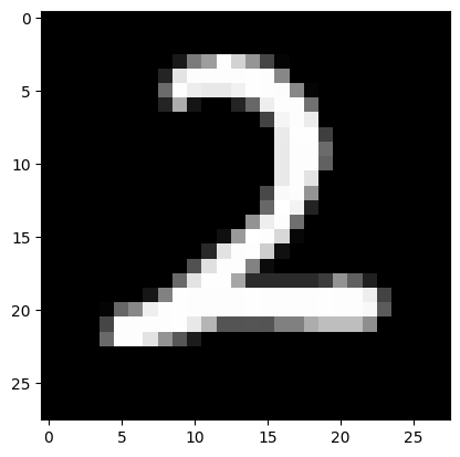
def test_prediction(index, W1, b1, W2, b2):
    current_image = X_train[:, index, None]
    prediction = make_predictions(X_train[:, index, None], W1, b1, W2, b2)
    label = Y_train[index]
    print("Prediction: ", prediction)
    print("Label: ", label)
    
    # change image data from a vector of it's pixel values into matrix of it's values and set them back to values between 0 and 255 (instead of 0-1)
    current_image = current_image.reshape((28, 28)) * 255
    plt.gray()
    # show data as an image
    plt.imshow(current_image, interpolation='nearest')
    plt.show()

Let’s see a few examples.

test_prediction(0, W1, b1, W2, b2)
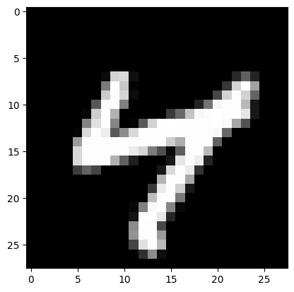
test_prediction(1, W1, b1, W2, b2)
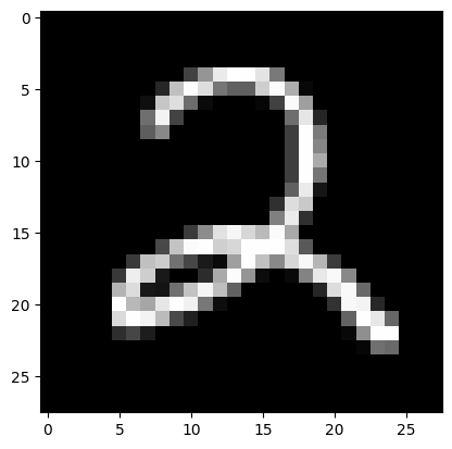
test_prediction(2, W1, b1, W2, b2)
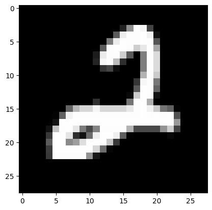
test_prediction(3, W1, b1, W2, b2)

Prediction:  [2]
Label:  2

png

Prediction:  [4]
Label:  4

png

Prediction:  [2]
Label:  2

png

Prediction:  [2]
Label:  2

png

Finally, let’s find the accuracy on the validation set:

dev_predictions = make_predictions(X_valid, W1, b1, W2, b2)
get_accuracy(dev_predictions, Y_valid)

[2 1 8 3 8 4 8 3 5 4 8 4 3 0 8 0 1 8 3 6 7 7 2 6 5 8 2 8 1 0 5 7 2 3 0 8 7
4 9 5 6 3 1 0 5 9 7 2 1 5 5 4 9 9 3 2 2 2 5 3 6 9 2 3 6 0 2 8 1 1 7 0 6
0 0 2 9 4 1 5 4 7 0 8 2 7 4 3 7 9 5 5 7 7 1 8 1 0 8 6 1 6 2 1 4 2 7 6 7
7 5 0 3 5 5 4 5 1 8 0 5 3 9 6 5 2 1 5 3 7 3 9 2 6 8 6 1 1 8 6 7 6 2 6 6
0 7 3 3 4 9 0 3 1 1 5 4 4 5 3 3 9 3 2 1 2 9 8 9 7 0 7 7 9 2 4 0 9 2 3 6
0 4 5 9 5 3 7 5 4 7 8 3 0 7 7 0 8 9 2 6 3 5 5 8 8 6 7 2 1 7 3 6 1 3 1 6
1 4 3 4 5 4 8 9 4 3 8 3 9 3 3 1 2 7 8 0 7 9 7 2 2 7 7 6 2 5 8 1 9 8 3 0
0 5 6 8 7 3 7 4 3 0 1 9 1 3 4 0 9 6 9 7 9 9 5 9 5 5 1 4 0 9 0 6 5 1 0 6
3 8 6 9 2 1 8 4 4 0 4 1 2 6 1 2 0 1 2 4 6 2 8 7 2 5 6 7 3 7 4 2 0 9 3 5
2 1 1 3 4 4 1 9 9 5 3 3 8 1 9 0 4 0 2 5 8 2 2 3 9 0 7 2 7 2 2 5 0 8 2 2
2 6 7 4 6 6 5 3 8 5 2 6 3 3 3 1 7 1 5 1 6 2 9 2 2 7 3 7 4 0 5 3 5 9 9 1
7 9 8 5 2 3 5 6 6 3 7 8 1 0 8 9 7 0 8 4 6 6 6 5 6 9 3 6 8 4 4 1 0 9 1 0
1 8 7 3 3 6 7 5 0 2 6 1 4 7 5 6 7 4 4 3 2 0 0 6 6 5 1 3 9 0 5 4 2 8 6 4
3 4 6 0 0 1 0 6 5 0 8 3 7 1 8 5 6 4 1 7 8 6 7 3 5 6 0 3 3 5 2 8 1 4 2 9
4 2 0 8 7 2 3 6 6 1 3 9 3 1 6 1 1 9 2 9 6 7 2 4 1 0 9 1 6 5 2 4 0 8 4 6
2 7 0 6 8 4 6 6 6 8 1 1 7 9 0 0 6 9 7 8 4 1 7 8 2 3 4 9 7 4 7 2 9 2 2 1
5 0 6 9 3 6 7 5 9 8 5 2 7 3 9 4 8 9 7 8 0 0 6 3 0 8 3 5 5 7 1 8 1 1 1 8
3 4 2 4 6 2 4 9 7 2 6 9 3 5 2 4 5 1 1 9 6 5 7 7 6 1 3 9 7 2 1 4 4 1 0 6
8 1 0 8 6 5 9 4 6 9 8 6 2 1 0 1 5 7 1 5 8 9 5 1 3 1 2 7 7 8 5 6 2 4 0 6
5 9 6 8 0 4 3 0 3 3 3 3 7 5 8 5 1 5 1 7 0 8 0 4 6 0 1 1 7 1 4 3 7 1 8 9
2 5 8 4 4 4 0 7 9 1 8 1 2 6 6 9 4 4 3 9 4 7 9 0 8 1 9 9 2 0 7 0 6 4 3 1
5 8 1 6 7 6 7 0 7 4 8 5 3 3 6 4 4 7 4 1 1 5 0 5 5 3 8 9 5 2 6 5 6 9 3 3
4 9 5 0 2 2 4 4 2 3 7 3 2 5 9 2 3 2 6 1 2 8 7 5 9 1 9 4 8 5 9 3 7 1 8 7
6 9 9 2 3 4 4 0 3 2 2 3 8 7 3 2 1 0 7 0 1 3 1 5 5 5 3 7 0 4 8 8 3 6 9 4
4 7 3 3 6 7 9 9 5 8 7 6 0 9 7 0 1 3 9 5 1 8 9 8 1 2 8 9 4 2 5 7 8 2 3 4
6 6 3 1 0 3 7 9 6 7 3 7 5 2 7 3 6 6 7 9 4 9 0 4 7 0 4 3 0 7 2 1 4 0 8 6
6 4 7 0 1 6 8 3 4 8 1 2 4 5 4 3 8 6 2 9 9 5 1 4 0 2 8 5 6 9 4 8 3 1 9 8
 5] [2 1 8 3 8 9 0 3 5 4 8 4 3 0 8 0 1 3 3 6 7 7 2 6 0 8 8 8 1 0 5 7 2 3 0 8 9
4 4 2 6 3 3 0 8 7 7 2 1 5 6 6 9 8 3 2 2 3 5 3 6 9 4 3 6 0 2 8 1 1 7 0 6
0 0 2 9 4 1 3 4 9 3 5 3 7 4 3 7 9 5 5 7 0 1 8 1 0 4 6 3 6 2 1 4 2 7 6 7
7 5 0 5 5 5 4 5 1 8 0 3 3 9 6 5 2 1 3 3 7 3 9 2 6 8 2 1 1 8 6 7 6 2 6 6
0 7 3 3 4 9 9 3 1 1 5 4 4 5 5 3 4 3 2 2 2 9 8 9 7 0 7 7 9 2 4 5 9 8 5 6
0 4 5 9 8 3 7 5 9 7 8 3 0 7 7 0 5 9 2 6 3 3 5 8 8 5 7 2 1 7 3 6 1 3 1 6
1 5 3 4 5 4 8 9 4 3 8 5 4 3 3 1 2 7 8 0 7 9 7 2 2 7 9 6 1 5 8 1 8 3 3 0
0 5 6 8 7 9 7 2 5 0 1 9 1 3 4 0 1 6 7 7 9 7 6 9 5 5 1 4 0 9 0 0 5 1 0 6
3 8 6 9 2 1 8 5 4 0 4 1 2 6 1 2 0 1 2 4 6 2 8 7 2 3 6 7 3 7 9 2 0 9 5 3
2 1 1 2 4 4 1 9 9 5 3 3 8 1 9 0 4 0 2 5 8 2 2 3 9 0 7 5 7 2 2 5 2 8 2 2
2 2 7 4 6 6 5 3 8 5 2 6 3 5 3 1 7 1 5 1 6 2 9 2 2 7 3 7 4 0 5 3 5 9 4 1
7 9 8 5 4 3 5 6 6 3 9 8 1 5 8 7 7 0 8 2 6 6 6 5 6 9 3 6 3 4 4 1 0 9 1 0
1 8 7 5 3 6 7 5 0 2 6 1 4 7 5 6 7 4 4 5 2 0 0 0 6 5 1 3 9 0 5 4 2 3 6 4
3 4 6 0 0 1 0 6 5 3 3 3 7 1 6 3 2 4 1 7 8 6 7 3 5 6 0 3 3 5 2 8 1 4 2 9
4 2 0 8 7 2 8 6 6 1 3 9 3 1 6 1 1 9 2 4 6 7 5 4 1 0 9 1 6 5 2 4 0 8 4 6
2 7 0 6 8 4 6 0 6 8 1 1 7 9 0 0 6 4 7 8 4 1 9 8 2 3 4 7 7 5 7 2 9 2 2 1
5 0 6 7 5 6 7 5 3 8 3 7 7 3 9 4 8 9 7 4 0 0 6 2 0 8 3 5 5 7 1 8 1 3 1 8
3 4 1 4 6 2 4 8 7 2 6 9 3 5 2 9 5 1 1 4 6 3 7 7 6 1 3 9 7 8 1 4 4 1 0 6
8 1 5 8 6 4 7 4 6 9 3 6 2 1 0 1 5 7 1 5 8 9 5 1 3 1 2 7 9 8 5 6 2 4 0 6
5 9 6 8 2 4 8 0 3 3 3 8 7 8 8 0 1 5 1 7 0 8 0 4 6 0 1 1 9 3 4 3 7 1 8 9
9 8 8 4 4 4 0 7 9 1 8 9 4 6 8 7 4 4 8 9 4 9 9 0 8 1 9 9 2 0 7 0 6 9 3 1
5 8 1 6 3 6 7 0 7 9 8 5 3 3 2 9 4 7 4 1 8 5 0 5 5 5 8 9 5 9 6 9 6 9 3 3
4 9 5 0 2 2 4 4 2 8 7 3 3 3 1 2 3 2 6 1 8 8 7 5 5 1 9 4 8 5 9 3 1 1 8 7
6 9 9 3 3 4 4 0 3 3 2 9 8 7 3 2 1 0 7 0 1 3 1 5 5 5 3 2 5 9 8 5 9 6 9 4
4 7 3 3 6 7 9 9 3 5 7 6 0 9 7 0 1 3 9 5 1 5 9 8 1 2 8 9 4 2 5 7 2 2 3 4
6 6 3 1 0 3 7 7 6 7 8 7 5 3 7 3 6 6 7 7 4 7 0 4 7 0 7 3 0 7 2 1 4 0 8 6
6 4 7 0 1 6 8 3 6 8 1 2 4 6 4 3 3 6 2 4 7 5 1 4 0 2 8 5 6 9 4 2 3 8 9 8
 3]





83

83% accuracy. So our model generalised from the training data pretty well.

Conclusion

So as far as understanding the underlying maths of the back propagation part, I have to admit that I kind of took Samson’s word for it as I couldn’t find anymore detailed information other than what is here. I’m sure if I spend enough time that I would realise it is simply an application of gradients and the chain rule..

The key thing I took away from this exercise, was the importance of considering the shape of the data at each step. The amount of transposing (.T) that needed to be done was all for good reason. This particular attention towards how the data looks at each step is something I am sure I have neglected in my previous attempts at the MNIST digit recognizer Kaggle competition. Given time, I will go back to reassess my previous attempts and see if I can fix them by going through each step with an eye on the shape of the data…

Gurtaj's blog!

Introduction

ASIDE

The softmax function

The one_hot function

END ASIDE

ASIDE

END ASIDE

Conclusion

The `one_hot` function