Gurtaj's blog!

Introduction

After recently fixing some previous models that were broken (see the tl;dr section in this notebook to see where I had gone wrong previously) I decided to see if I can do the same with some other models. In this notebook I will attempt to fix my previous attempts at a 2 linear layer model using PyTorch Modules to construct the architecture and then utilising fastai’s Learner to create and train the model from this architecture.

TL;DR

The places where I was going wrong previously are as follows:

The output of this model was in a different orientation to that which was output by our more manual model.
- batch_accuracy and rmse were therefore edited accordingly in order to accomodate the differing shape
The DataLoader that I was creating, for our test/submission data, was not that which was expected by our Learner’s get_preds method when trying to make predictions on it.
- previously I was running test_dl = DataLoader(test_dset, batch_size=len(test_dset)), the fix was to access the dataset property of test_dset rather than trying to access test_dset directly: test_dl = DataLoader(test_dset.dataset, batch_size=len(test_dset))
- Whilst I was figuring out what was going wrong with the above I tried multiple different ways of using Learner’s predict method also, but in the end the above way of using get_preds worked.

# This Python 3 environment comes with many helpful analytics libraries installed
# It is defined by the kaggle/python Docker image: https://github.com/kaggle/docker-python
# For example, here's several helpful packages to load

import numpy as np # linear algebra
import pandas as pd # data processing, CSV file I/O (e.g. pd.read_csv)

# Input data files are available in the read-only "../input/" directory
# For example, running this (by clicking run or pressing Shift+Enter) will list all files under the input directory

import os
for dirname, _, filenames in os.walk('/kaggle/input'):
    for filename in filenames:
        print(os.path.join(dirname, filename))

# You can write up to 20GB to the current directory (/kaggle/working/) that gets preserved as output when you create a version using "Save & Run All" 
# You can also write temporary files to /kaggle/temp/, but they won't be saved outside of the current session

# install fastkaggle if not available
try: import fastkaggle
except ModuleNotFoundError:
    !pip install -Uq fastkaggle

from fastkaggle import *

comp = 'digit-recognizer'

path = setup_comp(comp, install='fastai "timm>=0.6.2.dev0"')

Warning: Your Kaggle API key is readable by other users on this system! To fix this, you can run 'chmod 600 /Users/gaz/.kaggle/kaggle.json'

from fastai.vision.all import *

path.ls()

(#3) [Path('digit-recognizer/test.csv'),Path('digit-recognizer/train.csv'),Path('digit-recognizer/sample_submission.csv')]

df = pd.read_csv(path/'train.csv')
df

	label	pixel0	pixel1	pixel2	pixel3	pixel4	pixel5	pixel6	pixel7	pixel8	...	pixel774	pixel775	pixel776	pixel777	pixel778	pixel779	pixel780	pixel781	pixel782	pixel783
0	1	0	0	0	0	0	0	0	0	0	...	0	0	0	0	0	0	0	0	0	0
1	0	0	0	0	0	0	0	0	0	0	...	0	0	0	0	0	0	0	0	0	0
2	1	0	0	0	0	0	0	0	0	0	...	0	0	0	0	0	0	0	0	0	0
3	4	0	0	0	0	0	0	0	0	0	...	0	0	0	0	0	0	0	0	0	0
4	0	0	0	0	0	0	0	0	0	0	...	0	0	0	0	0	0	0	0	0	0
...	...	...	...	...	...	...	...	...	...	...	...	...	...	...	...	...	...	...	...	...	...
41995	0	0	0	0	0	0	0	0	0	0	...	0	0	0	0	0	0	0	0	0	0
41996	1	0	0	0	0	0	0	0	0	0	...	0	0	0	0	0	0	0	0	0	0
41997	7	0	0	0	0	0	0	0	0	0	...	0	0	0	0	0	0	0	0	0	0
41998	6	0	0	0	0	0	0	0	0	0	...	0	0	0	0	0	0	0	0	0	0
41999	9	0	0	0	0	0	0	0	0	0	...	0	0	0	0	0	0	0	0	0	0

42000 rows × 785 columns

train_data_split = df.iloc[:33_600,:]
valid_data_split = df.iloc[33_600:,:]

len(train_data_split)/42000,len(valid_data_split)/42000

(0.8, 0.2)

pixel_value_columns = train_data_split.iloc[:,1:]
label_value_column = train_data_split.iloc[:,:1]

pixel_value_columns = pixel_value_columns.apply(lambda x: x/255)
train_data = pd.concat([label_value_column, pixel_value_columns], axis=1)

train_data.describe()

	label	pixel0	pixel1	pixel2	pixel3	pixel4	pixel5	pixel6	pixel7	pixel8	...	pixel774	pixel775	pixel776	pixel777	pixel778	pixel779	pixel780	pixel781	pixel782	pixel783
count	33600.000000	33600.0	33600.0	33600.0	33600.0	33600.0	33600.0	33600.0	33600.0	33600.0	...	33600.000000	33600.000000	33600.000000	33600.000000	33600.000000	33600.000000	33600.0	33600.0	33600.0	33600.0
mean	4.459881	0.0	0.0	0.0	0.0	0.0	0.0	0.0	0.0	0.0	...	0.000801	0.000454	0.000255	0.000086	0.000037	0.000007	0.0	0.0	0.0	0.0
std	2.885525	0.0	0.0	0.0	0.0	0.0	0.0	0.0	0.0	0.0	...	0.024084	0.017751	0.013733	0.007516	0.005349	0.001326	0.0	0.0	0.0	0.0
min	0.000000	0.0	0.0	0.0	0.0	0.0	0.0	0.0	0.0	0.0	...	0.000000	0.000000	0.000000	0.000000	0.000000	0.000000	0.0	0.0	0.0	0.0
25%	2.000000	0.0	0.0	0.0	0.0	0.0	0.0	0.0	0.0	0.0	...	0.000000	0.000000	0.000000	0.000000	0.000000	0.000000	0.0	0.0	0.0	0.0
50%	4.000000	0.0	0.0	0.0	0.0	0.0	0.0	0.0	0.0	0.0	...	0.000000	0.000000	0.000000	0.000000	0.000000	0.000000	0.0	0.0	0.0	0.0
75%	7.000000	0.0	0.0	0.0	0.0	0.0	0.0	0.0	0.0	0.0	...	0.000000	0.000000	0.000000	0.000000	0.000000	0.000000	0.0	0.0	0.0	0.0
max	9.000000	0.0	0.0	0.0	0.0	0.0	0.0	0.0	0.0	0.0	...	0.996078	0.996078	0.992157	0.992157	0.956863	0.243137	0.0	0.0	0.0	0.0

8 rows × 785 columns

pixel_value_columns_tensor = torch.tensor(train_data.iloc[:,1:].values).float()
label_value_column_tensor = torch.tensor(train_data.iloc[:,:1].values).float()

train_ds = list(zip(pixel_value_columns_tensor,label_value_column_tensor))

We’ll make this a function, so that we can do the same again for our validation data.

train_dl = DataLoader(train_ds, batch_size=256)
train_xb,train_yb = first(train_dl)

train_xb.shape,train_xb.shape

(torch.Size([256, 784]), torch.Size([256, 784]))

def dataset_from_dataframe(dframe):
    pixel_value_columns = dframe.iloc[:,1:]
    label_value_column = dframe.iloc[:,:1]

    pixel_value_columns = pixel_value_columns.apply(lambda x: x/255)

    pixel_value_columns_tensor = torch.tensor(train_data.iloc[:,1:].values).float()
    label_value_column_tensor = torch.tensor(train_data.iloc[:,:1].values).float()

    return list(zip(pixel_value_columns_tensor, label_value_column_tensor))

valid_ds = dataset_from_dataframe(valid_data_split)

valid_dl = DataLoader(valid_ds, batch_size=256)

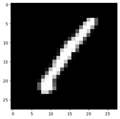
To ease my mind and help spot places where I could be making errors, i’ll make a function that can visually show a particular input (digit image) to me.

def show_image(item):
    item = item.view(28,28) * 255
    plt.gray()
    plt.imshow(item, interpolation='nearest')
    plt.show()

Now, for my sanity, i’ll test an images in train_xb.

show_image(train_xb[0])

png

Loss Function

number_of_classes = 10

def one_hot(yb):
    batch_size = len(yb)
    one_hot_yb = torch.zeros(batch_size, number_of_classes)
    x_coordinates_array = torch.arange(len(one_hot_yb))
    # used `.squeeze()` becasue yb originally has the size (batch_size, 1) and we just want a size of (batch_size). ([1, 2, 3, ...] instead of [[1], [2], [3], ...])
    # used `.long()` because: "tensors used as indices must be long, int, byte or bool tensors"
    y_coordinates_array = yb.squeeze().long()
    # set to `1.` rather than `1` because: Index put requires the source and destination dtypes match, got Float for the destination and Long for the source.
    one_hot_yb[x_coordinates_array, y_coordinates_array] = torch.tensor(1.)
    
    return one_hot_yb.T

def rmse(a, b):
    b = one_hot(b)
    mse = nn.MSELoss()
    loss = torch.sqrt(mse(a, b))
    
    return loss

one_hot(train_yb),one_hot(train_yb).shape,one_hot(train_yb)[:,0],train_yb[0]

(tensor([[0., 1., 0.,  ..., 0., 0., 0.],
         [1., 0., 1.,  ..., 0., 0., 1.],
         [0., 0., 0.,  ..., 0., 0., 0.],
         ...,
         [0., 0., 0.,  ..., 0., 1., 0.],
         [0., 0., 0.,  ..., 0., 0., 0.],
         [0., 0., 0.,  ..., 0., 0., 0.]]),
 torch.Size([10, 256]),
 tensor([0., 1., 0., 0., 0., 0., 0., 0., 0., 0.]),
 tensor([1.]))

Let’s run it on our test batch predictions from above.

Trainability

def calc_grad(batch_inputs, batch_labels, batch_model):
    batch_preds = batch_model(batch_inputs)
    loss = rmse(batch_preds, batch_labels)
    loss.backward()

def train_epoch(dl, batch_model, params, lr):
    for xb,yb in dl:
        calc_grad(xb, yb, batch_model)
        for p in params:
            pdata1 = p.data
            p.data -= p.grad*lr
            pdata2 = p.data
            p.grad.zero_()

Validation and Metric

def get_predicted_label(pred):
    #returns index of highest value in tensor, which convenietnly also is directly the the digit/label that it corresponds to
    return torch.argmax(pred)

get_predicted_label(torch.tensor([0,4,3,2,6,1]))

tensor(4)

Accuracy

def batch_accuracy(preds, yb):
    #remember each column in our preds is an indivudual prediction, so we transpose preds in order to iterate through each precition in our list comprehension below
    preds = torch.tensor([get_predicted_label(pred) for pred in preds.T])
    # is_correct is a tensor of True and False values
    is_correct = preds==yb.squeeze()
    # now we turn all True values into 1 and all False values into 0, then return the mean of those values
    return is_correct.float().mean()

def validate_epoch(dl, batch_model):
    accuracies = [batch_accuracy(batch_model(xb),yb) for xb,yb in dl]
    # turn list of tensors into one single tensor of stacked values, so that we can then calculate the mean across all those values
    stacked_tensor = torch.stack(accuracies)
    mean_tensor = stacked_tensor.mean()
    # round method only works on value within tensor so we use item() to get it (and then round to four decimal places)
    return round(mean_tensor.item(), 4)

Using Pytorch’s nn Modules

Create Architecture

Lets create our model architecture using PyTorch modules for our Linear and ReLU layers, and we then we we can take advatage of fastai’s Learner module and SGD (Stochastic Gradient Descent) optimiser for our training. Perhaps that will show even further improvements.

simple_net = nn.Sequential(
    nn.Linear(784,30),
    nn.ReLU(),
    nn.Linear(30,10)
)

Note how we do not need to initialise the params manually here, we just pass the desired shapes of our params to nn.Linear and it initialises them internally.

Some Changes Made

After a bit of experimentation with this method I noticed that the predictions/output of simple_net (see previous notebook) were not in the same shape as with simple_nn (without use of the Pytorch nn Modules), rather they were the in the transposed format. For that reason I have ammended batch_accuracy and rmse to include the relevant pieces of data augmentation needed (see relevant comments in the code itself).

def batch_accuracy(preds, yb):
    # preds no longer needs to e transposed like it was before
    preds = torch.tensor([get_predicted_label(pred) for pred in preds])
    # is_correct is a tensor of True and False values
    is_correct = preds==yb.squeeze()
    # now we turn all True values into 1 and all False values into 0, then return the mean of those values
    return is_correct.float().mean()

def rmse(a, b):
    # the one hot encoded labels needed transposing to match the shape of the predictions/outputs of `simple_net`
    b = one_hot(b.squeeze()).T
    mse = nn.MSELoss()
    loss = torch.sqrt(mse(a, b))
    
    return loss

### End of Changes Made

Create Learner

dls = DataLoaders(train_dl,valid_dl)

learn = Learner(dls, simple_net, opt_func=SGD,
                loss_func=rmse, metrics=batch_accuracy)

Training Model

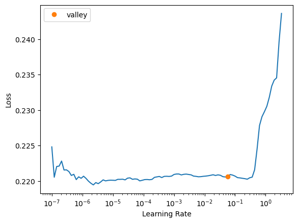
Learner contains the very handy lr_find() method that runs through all possible lr values and locates the ‘sweet spot’ for it’s value. This saves us having to manually triall and error different values ourselves!

learn.lr_find()

SuggestedLRs(valley=0.05754399299621582)

png

learn.fit(10, lr=0.01)

epoch	train_loss	valid_loss	batch_accuracy	time
0	0.306814	0.295378	0.269286	00:00
1	0.285192	0.279350	0.501577	00:00
2	0.272066	0.267298	0.623780	00:00
3	0.260594	0.256262	0.698631	00:01
4	0.250645	0.246955	0.737024	00:01
5	0.242500	0.239447	0.761756	00:00
6	0.235948	0.233414	0.777887	00:00
7	0.230643	0.228504	0.789018	00:00
8	0.226261	0.224414	0.797976	00:00
9	0.222562	0.220934	0.805089	00:00

So with the same lr (learning rate) as simple_nn we have acheived an ~81.3 % accuracy but this time in just 10 epochs.

Submision

We can load the test data directly into learn and then use it to make our predictions on that data.

Notice how we didn’t include the final step of creating a dataloader here, like we did for our training and validation data earlier. That’s because, for some reason, we now need to use the test_dl method on the dls object of our learn. I think it is something to do with how I have done this all manaully in a way that we normally wouldn’t in real practice. (for the sake of learning). For example there is the fact that I earlier used DataLoader on the training and validation data instead of ImageDataLoaders or DataBlock with the appropriate input and output types declared (ImageBlock and CategoryBlock respectively).

The methods used below were acquired from this comment in the fastai forums.

test_df = pd.read_csv(path/'test.csv')

test_df.describe()

	pixel0	pixel1	pixel2	pixel3	pixel4	pixel5	pixel6	pixel7	pixel8	pixel9	...	pixel774	pixel775	pixel776	pixel777	pixel778	pixel779	pixel780	pixel781	pixel782	pixel783
count	28000.0	28000.0	28000.0	28000.0	28000.0	28000.0	28000.0	28000.0	28000.0	28000.0	...	28000.000000	28000.000000	28000.000000	28000.000000	28000.000000	28000.0	28000.0	28000.0	28000.0	28000.0
mean	0.0	0.0	0.0	0.0	0.0	0.0	0.0	0.0	0.0	0.0	...	0.164607	0.073214	0.028036	0.011250	0.006536	0.0	0.0	0.0	0.0	0.0
std	0.0	0.0	0.0	0.0	0.0	0.0	0.0	0.0	0.0	0.0	...	5.473293	3.616811	1.813602	1.205211	0.807475	0.0	0.0	0.0	0.0	0.0
min	0.0	0.0	0.0	0.0	0.0	0.0	0.0	0.0	0.0	0.0	...	0.000000	0.000000	0.000000	0.000000	0.000000	0.0	0.0	0.0	0.0	0.0
25%	0.0	0.0	0.0	0.0	0.0	0.0	0.0	0.0	0.0	0.0	...	0.000000	0.000000	0.000000	0.000000	0.000000	0.0	0.0	0.0	0.0	0.0
50%	0.0	0.0	0.0	0.0	0.0	0.0	0.0	0.0	0.0	0.0	...	0.000000	0.000000	0.000000	0.000000	0.000000	0.0	0.0	0.0	0.0	0.0
75%	0.0	0.0	0.0	0.0	0.0	0.0	0.0	0.0	0.0	0.0	...	0.000000	0.000000	0.000000	0.000000	0.000000	0.0	0.0	0.0	0.0	0.0
max	0.0	0.0	0.0	0.0	0.0	0.0	0.0	0.0	0.0	0.0	...	253.000000	254.000000	193.000000	187.000000	119.000000	0.0	0.0	0.0	0.0	0.0

8 rows × 784 columns

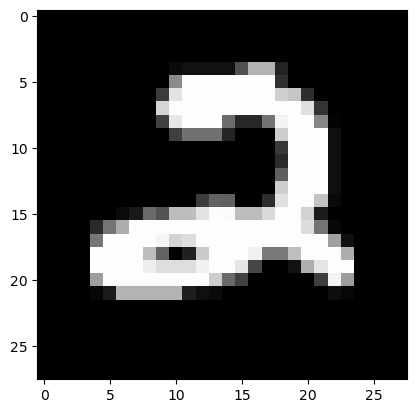
tense = torch.tensor(test_df.values)/255

show_image(tense[0])

png

# learn.predict(tense)

pixel_value_columns = torch.tensor(test_df.values)/255

pixel_value_columns_tensor = torch.tensor(pixel_value_columns).float()
dummy_label_value_column_tensor = torch.zeros(len(pixel_value_columns_tensor)).float()

test_list = list(zip(pixel_value_columns_tensor, dummy_label_value_column_tensor))

/var/folders/8z/yl3fjfvj4872y8z3xmr4dr2c0000gn/T/ipykernel_50580/2487244240.py:3: UserWarning: To copy construct from a tensor, it is recommended to use sourceTensor.clone().detach() or sourceTensor.clone().detach().requires_grad_(True), rather than torch.tensor(sourceTensor).
  pixel_value_columns_tensor = torch.tensor(pixel_value_columns).float()

test_dset = DataLoader(test_list)

In my previous attempt, I was loading in the test set as a DataLoader using the following method on our Learner.

# test_dl = learn.dls.test_dl(test_dset, num_workers=0, shuffle=False)

test_dl = DataLoader(test_dset.dataset, batch_size=len(test_dset))

test_xb,test_yb = first(test_dl)
test_xb.shape,test_yb.shape

(torch.Size([28000, 784]), torch.Size([28000]))

show_image(test_xb[0]),test_yb[0]

png

(None, tensor(0.))

Let’s now look at the output of our model

preds = learn.get_preds(dl=test_dl)

x,y = preds
x[0],y[0]

(tensor([ 0.3201,  0.0867,  0.8190,  0.0424, -0.0170, -0.2212,  0.0148, -0.0009,
          0.1567, -0.0841]),
 tensor(0.))

looks like we are getting tuples as our output. The first item in each tuple, x is likely to be the activation that corresponds to each possible class that we are classifying our inputs by (each possible digit).

The second item in each tuple, y, I now realise is the labels that we provided in the test dataset, which were all zeros.

Let’s print a few tuple pairs to confirm this.

x is our prediction activations now and y is the labels we supplied which are just 0s. Let’s convert our prediction activations into predicted labels.

get_predicted_label(x[0]),y[0],get_predicted_label(x[1]),y[1],get_predicted_label(x[2]),y[2],get_predicted_label(x[3]),y[3]

(tensor(2),
 tensor(0.),
 tensor(0),
 tensor(0.),
 tensor(9),
 tensor(0.),
 tensor(7),
 tensor(0.))

Yep, seems we were right. And since the index of the activations corresponds to the actual values of our classes (0-9) we can just use get_predicted_label to get our predicted labels. So let’s get our submission data ready. First, we get a list of our single value predictions, using a list comprehension.

predicted_labels = [get_predicted_label(pred).numpy() for pred in x]

predicted_labels_series = pd.Series(predicted_labels, name="Label")

predicted_labels_series

      2
      0
      9
      7
      3
        ..
  9
  7
  3
  9
  2
Name: Label, Length: 28000, dtype: object

sample_submission = pd.read_csv(path/'sample_submission.csv')

sample_submission

	ImageId	Label
0	1	0
1	2	0
2	3	0
3	4	0
4	5	0
...	...	...
27995	27996	0
27996	27997	0
27997	27998	0
27998	27999	0
27999	28000	0

28000 rows × 2 columns

sample_submission['Label'] = predicted_labels_series

sample_submission

	ImageId	Label
0	1	2
1	2	0
2	3	9
3	4	7
4	5	3
...	...	...
27995	27996	9
27996	27997	7
27997	27998	3
27998	27999	9
27999	28000	2

28000 rows × 2 columns

sample_submission.to_csv('subm.csv', index=False)

!head subm.csv

ImageId,Label
1,2
2,0
3,9
4,7
5,3
6,7
7,0
8,3
9,0

!kaggle competitions submit -c digit-recognizer  -f ./subm.csv -m "two linear layer model using PyTorch nn.Linear and nn.ReLu UPDATED"

Warning: Your Kaggle API key is readable by other users on this system! To fix this, you can run 'chmod 600 /Users/gaz/.kaggle/kaggle.json'
100%|█████████████████████████████████████████| 208k/208k [00:00<00:00, 281kB/s]
Successfully submitted to Digit Recognizer

This received a score of 0.80389. This is not bad but also not our best. In fact, the 2 layer linear model without the use of PyTorch’s nn modules did better. You may have noticed that we didn’t actualy add soft max to our model architecture. Let’s try that now and see if we have any improvements.

With Softmax

simple_net = nn.Sequential(
    nn.Linear(784,30),
    nn.ReLU(),
    nn.Linear(30,10),
    nn.Softmax()
)

learn = Learner(dls, simple_net, opt_func=SGD,
                loss_func=rmse, metrics=batch_accuracy)

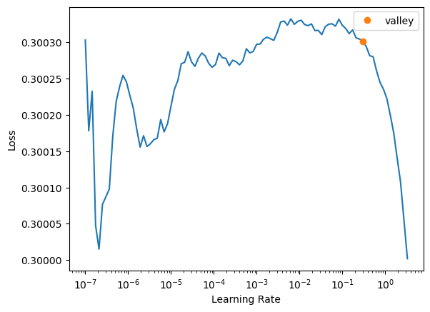
learn.lr_find()

/Users/gaz/mambaforge/envs/fastbook/lib/python3.10/site-packages/torch/nn/modules/container.py:217: UserWarning: Implicit dimension choice for softmax has been deprecated. Change the call to include dim=X as an argument.
  input = module(input)

SuggestedLRs(valley=0.3019951581954956)

png

learn.fit(10, lr=0.1)

epoch	train_loss	valid_loss	batch_accuracy	time
0	0.299001	0.298298	0.141042	00:01
1	0.296652	0.295476	0.219702	00:01
2	0.292797	0.290697	0.356131	00:01
3	0.285784	0.282168	0.512232	00:01
4	0.274211	0.268486	0.625684	00:01
5	0.257071	0.248983	0.715357	00:01
6	0.232951	0.222247	0.755595	00:01
7	0.207361	0.198186	0.776190	00:01
8	0.187238	0.180095	0.819732	00:01
9	0.171898	0.166387	0.846518	00:01

So with the same number of epochs we have now acheived an ~85 % accuracy, definitely an improvement upon not using nn.Softmax.

Submision

test_df = pd.read_csv(path/'test.csv')

test_df.describe()

	pixel0	pixel1	pixel2	pixel3	pixel4	pixel5	pixel6	pixel7	pixel8	pixel9	...	pixel774	pixel775	pixel776	pixel777	pixel778	pixel779	pixel780	pixel781	pixel782	pixel783
count	28000.0	28000.0	28000.0	28000.0	28000.0	28000.0	28000.0	28000.0	28000.0	28000.0	...	28000.000000	28000.000000	28000.000000	28000.000000	28000.000000	28000.0	28000.0	28000.0	28000.0	28000.0
mean	0.0	0.0	0.0	0.0	0.0	0.0	0.0	0.0	0.0	0.0	...	0.164607	0.073214	0.028036	0.011250	0.006536	0.0	0.0	0.0	0.0	0.0
std	0.0	0.0	0.0	0.0	0.0	0.0	0.0	0.0	0.0	0.0	...	5.473293	3.616811	1.813602	1.205211	0.807475	0.0	0.0	0.0	0.0	0.0
min	0.0	0.0	0.0	0.0	0.0	0.0	0.0	0.0	0.0	0.0	...	0.000000	0.000000	0.000000	0.000000	0.000000	0.0	0.0	0.0	0.0	0.0
25%	0.0	0.0	0.0	0.0	0.0	0.0	0.0	0.0	0.0	0.0	...	0.000000	0.000000	0.000000	0.000000	0.000000	0.0	0.0	0.0	0.0	0.0
50%	0.0	0.0	0.0	0.0	0.0	0.0	0.0	0.0	0.0	0.0	...	0.000000	0.000000	0.000000	0.000000	0.000000	0.0	0.0	0.0	0.0	0.0
75%	0.0	0.0	0.0	0.0	0.0	0.0	0.0	0.0	0.0	0.0	...	0.000000	0.000000	0.000000	0.000000	0.000000	0.0	0.0	0.0	0.0	0.0
max	0.0	0.0	0.0	0.0	0.0	0.0	0.0	0.0	0.0	0.0	...	253.000000	254.000000	193.000000	187.000000	119.000000	0.0	0.0	0.0	0.0	0.0

8 rows × 784 columns

tense = torch.tensor(test_df.values)/255

show_image(tense[0])

png

pixel_value_columns = torch.tensor(test_df.values)/255

pixel_value_columns_tensor = torch.tensor(pixel_value_columns).float()
dummy_label_value_column_tensor = torch.zeros(len(pixel_value_columns_tensor)).float()

test_list = list(zip(pixel_value_columns_tensor, dummy_label_value_column_tensor))

/var/folders/8z/yl3fjfvj4872y8z3xmr4dr2c0000gn/T/ipykernel_50580/2487244240.py:3: UserWarning: To copy construct from a tensor, it is recommended to use sourceTensor.clone().detach() or sourceTensor.clone().detach().requires_grad_(True), rather than torch.tensor(sourceTensor).
  pixel_value_columns_tensor = torch.tensor(pixel_value_columns).float()

test_dset = DataLoader(test_list)

test_dl = DataLoader(test_dset.dataset, batch_size=len(test_dset))

test_xb,test_yb = first(test_dl)
test_xb.shape,test_yb.shape

(torch.Size([28000, 784]), torch.Size([28000]))

show_image(test_xb[0]),test_yb[0]

png

(None, tensor(0.))

Let’s now look at the output of our model

preds = learn.get_preds(dl=test_dl)

x,y = preds
x[0],y[0]

/Users/gaz/mambaforge/envs/fastbook/lib/python3.10/site-packages/torch/nn/modules/container.py:217: UserWarning: Implicit dimension choice for softmax has been deprecated. Change the call to include dim=X as an argument.
  input = module(input)

(tensor([1.1154e-02, 8.0940e-05, 9.7530e-01, 7.2095e-04, 6.1947e-04, 1.4843e-03,
         4.3284e-03, 4.7975e-04, 5.3718e-03, 4.6172e-04]),
 tensor(0.))

Let’s confirm that softmax is doing what it is supposed to do. Our 10 activations, per image, should now add up to 1.

sum(x[0])

tensor(1.0000)

Looks good to go, let’s continue with our submission.

predicted_labels = [get_predicted_label(pred).numpy() for pred in x]

predicted_labels_series = pd.Series(predicted_labels, name="Label")

predicted_labels_series

      2
      0
      9
      7
      2
        ..
  9
  7
  3
  9
  2
Name: Label, Length: 28000, dtype: object

sample_submission = pd.read_csv(path/'sample_submission.csv')

sample_submission

	ImageId	Label
0	1	0
1	2	0
2	3	0
3	4	0
4	5	0
...	...	...
27995	27996	0
27996	27997	0
27997	27998	0
27998	27999	0
27999	28000	0

28000 rows × 2 columns

sample_submission['Label'] = predicted_labels_series

sample_submission

	ImageId	Label
0	1	2
1	2	0
2	3	9
3	4	7
4	5	2
...	...	...
27995	27996	9
27996	27997	7
27997	27998	3
27998	27999	9
27999	28000	2

28000 rows × 2 columns

sample_submission.to_csv('subm.csv', index=False)

!head subm.csv

ImageId,Label
1,2
2,0
3,9
4,7
5,2
6,7
7,0
8,3
9,0

!kaggle competitions submit -c digit-recognizer  -f ./subm.csv -m "two linear layer model using PyTorch nn.Linear and nn.ReLu with nn.Softmax UPDATED"

Warning: Your Kaggle API key is readable by other users on this system! To fix this, you can run 'chmod 600 /Users/gaz/.kaggle/kaggle.json'
100%|█████████████████████████████████████████| 208k/208k [00:00<00:00, 262kB/s]
Successfully submitted to Digit Recognizer

This received a score of 0.8485 an improvement upon the previous model by including softmax, as expected. The reason these two models didn’t get as good as the model that didn’t use PyTorch’s nn modules is likely becuase we used 500 epochs to train that one, whereas we only used 10 epochs to train the ones in this notebook. I didn’t want to risk overfitting but let’s try a few more epochs.

learn.fit(10, lr=0.1)

epoch	train_loss	valid_loss	batch_accuracy	time
0	0.159544	0.156210	0.862946	00:01
1	0.151786	0.148674	0.872202	00:01
2	0.145487	0.142968	0.879107	00:00
3	0.140583	0.138521	0.884732	00:01
4	0.136697	0.134954	0.888958	00:00
5	0.133540	0.132022	0.893631	00:01
6	0.130916	0.129555	0.896518	00:01
7	0.128688	0.127443	0.899315	00:01
8	0.126764	0.125600	0.901488	00:01
9	0.125074	0.123970	0.903036	00:01

/Users/gaz/mambaforge/envs/fastbook/lib/python3.10/site-packages/torch/nn/modules/container.py:217: UserWarning: Implicit dimension choice for softmax has been deprecated. Change the call to include dim=X as an argument.
  input = module(input)

So now after 20 epochs we have the same accuracy on our training data that we did on the 2 layer linear model that didn’t use PyTorch modules or fastai.

test_df = pd.read_csv(path/'test.csv')

tense = torch.tensor(test_df.values)/255

pixel_value_columns = torch.tensor(test_df.values)/255

pixel_value_columns_tensor = torch.tensor(pixel_value_columns).float()
dummy_label_value_column_tensor = torch.zeros(len(pixel_value_columns_tensor)).float()

test_list = list(zip(pixel_value_columns_tensor, dummy_label_value_column_tensor))

/var/folders/8z/yl3fjfvj4872y8z3xmr4dr2c0000gn/T/ipykernel_50580/2487244240.py:3: UserWarning: To copy construct from a tensor, it is recommended to use sourceTensor.clone().detach() or sourceTensor.clone().detach().requires_grad_(True), rather than torch.tensor(sourceTensor).
  pixel_value_columns_tensor = torch.tensor(pixel_value_columns).float()

test_dset = DataLoader(test_list)

test_dl = DataLoader(test_dset.dataset, batch_size=len(test_dset))

test_xb,test_yb = first(test_dl)
test_xb.shape,test_yb.shape

(torch.Size([28000, 784]), torch.Size([28000]))

Let’s now look at the output of our model

preds = learn.get_preds(dl=test_dl)

x,y = preds
x[0],y[0]

/Users/gaz/mambaforge/envs/fastbook/lib/python3.10/site-packages/torch/nn/modules/container.py:217: UserWarning: Implicit dimension choice for softmax has been deprecated. Change the call to include dim=X as an argument.
  input = module(input)

(tensor([2.0435e-04, 6.7201e-08, 9.9963e-01, 2.3687e-05, 1.7624e-07, 1.5268e-06,
         1.7885e-05, 1.3268e-06, 1.1589e-04, 2.1377e-06]),
 tensor(0.))

sum(x[0])

tensor(1.)

predicted_labels = [get_predicted_label(pred).numpy() for pred in x]

predicted_labels_series = pd.Series(predicted_labels, name="Label")

sample_submission = pd.read_csv(path/'sample_submission.csv')

sample_submission

	ImageId	Label
0	1	0
1	2	0
2	3	0
3	4	0
4	5	0
...	...	...
27995	27996	0
27996	27997	0
27997	27998	0
27998	27999	0
27999	28000	0

28000 rows × 2 columns

sample_submission['Label'] = predicted_labels_series

sample_submission

	ImageId	Label
0	1	2
1	2	0
2	3	9
3	4	9
4	5	2
...	...	...
27995	27996	9
27996	27997	7
27997	27998	3
27998	27999	9
27999	28000	2

28000 rows × 2 columns

sample_submission.to_csv('subm.csv', index=False)

!head subm.csv

ImageId,Label
1,2
2,0
3,9
4,9
5,2
6,7
7,0
8,3
9,0

!kaggle competitions submit -c digit-recognizer  -f ./subm.csv -m "two linear layer model using PyTorch nn.Linear and nn.ReLu with nn.Softmax UPDATED"

Warning: Your Kaggle API key is readable by other users on this system! To fix this, you can run 'chmod 600 /Users/gaz/.kaggle/kaggle.json'
100%|█████████████████████████████████████████| 208k/208k [00:00<00:00, 276kB/s]
Successfully submitted to Digit Recognizer

This got a score of 0.90078. Almost the same now as what we got (0.90142) after 500 epochs of training our 2 layer linear model using more manual PyTorch methods. There is an even more effective training method called 1cycle training that we will investigate below.

1cycle Training

Lets try the exact same model but now instead of using the fit methon on our Learner object, we will use fit_one_cycle.

So with fit_one_cycle instead of using a static learning rate, we actually have it as being dynamic over the course of the epoch:

start with low learning rate, since we don’t want the model to instantly diverge
end with low learning rate also, since we don’t want to jump over our point of minimum
ramp the learning rate up, and then back down, in between the start and end.

By training with higher learning rates (in between start and end), we:

train faster — a phenomenon named super-convergence.
we overfit less because we skip over the sharp local minima to end up in a smoother (and therefore more generalizable) part of the loss.

This type of training is called 1cycle training.

We will have to reinitialise our Learner.

learn = Learner(dls, simple_net, opt_func=SGD,
                loss_func=rmse, metrics=batch_accuracy)

learn.fit_one_cycle(1)

epoch	train_loss	valid_loss	batch_accuracy	time
0	0.124147	0.123946	0.903095	00:01

/Users/gaz/mambaforge/envs/fastbook/lib/python3.10/site-packages/torch/nn/modules/container.py:217: UserWarning: Implicit dimension choice for softmax has been deprecated. Change the call to include dim=X as an argument.
  input = module(input)

~90% accuracy in just one epoch! the efficiency of training has improved even further this time.

Let’s use this model to make predictions on the test data and make another submission to the competition.

x,y = learn.get_preds(dl=test_dl)

predicted_labels = [get_predicted_label(pred).numpy() for pred in x]

predicted_labels_series = pd.Series(predicted_labels, name="Label")

sample_submission = pd.read_csv(path/'sample_submission.csv')

sample_submission

	ImageId	Label
0	1	0
1	2	0
2	3	0
3	4	0
4	5	0
...	...	...
27995	27996	0
27996	27997	0
27997	27998	0
27998	27999	0
27999	28000	0

28000 rows × 2 columns

sample_submission['Label'] = predicted_labels_series

sample_submission

	ImageId	Label
0	1	2
1	2	0
2	3	9
3	4	9
4	5	2
...	...	...
27995	27996	9
27996	27997	7
27997	27998	3
27998	27999	9
27999	28000	2

28000 rows × 2 columns

sample_submission.to_csv('subm.csv', index=False)

!head subm.csv

ImageId,Label
1,2
2,0
3,9
4,9
5,2
6,7
7,0
8,3
9,0

!kaggle competitions submit -c digit-recognizer  -f ./subm.csv -m "two linear layer model using PyTorch nn.Linear and nn.ReLu with nn.Softmax with fit_one_cycle instead of fit (1cycle training)"

Warning: Your Kaggle API key is readable by other users on this system! To fix this, you can run 'chmod 600 /Users/gaz/.kaggle/kaggle.json'
100%|█████████████████████████████████████████| 208k/208k [00:00<00:00, 320kB/s]
Successfully submitted to Digit Recognizer

predictions_list = [int(pred.numpy()[0]) for pred in y]

---------------------------------------------------------------------------

IndexError                                Traceback (most recent call last)

Cell In[165], line 1
----> 1 predictions_list = [int(pred.numpy()[0]) for pred in y]

Cell In[165], line 1, in <listcomp>(.0)
----> 1 predictions_list = [int(pred.numpy()[0]) for pred in y]

IndexError: too many indices for array: array is 0-dimensional, but 1 were indexed

pred_labels = pd.Series(predictions_list, name="Label")

pred_labels

sample_submission = pd.read_csv(path/'sample_submission.csv')

sample_submission

sample_submission.to_csv('subm.csv', index=False)

!head subm.csv

sample_submission['Label'] = pred_labels

sample_submission

!kaggle competitions submit -c digit-recognizer  -f ./subm.csv -m "two linear layer model using PyTorch nn.Linear and nn.ReLu and nn.Softmax, trained for 10 epochs."

A score of 0.90078 once again but this time with just one epoch of training. 1cycle training is clearly a very efficient way to train models.

Conclusion

Previously I have learnt that looking at how our data looks, along each step of our processing is very important, this notebook has reinforced that and also stressed the fast that this is just as important for the test/submission data as it is for our training data. I’ve also learnt that there are multiple methods on Learner that we can use for making predictions and that I don’t quite yet understand which is better of if there are select specific reasons to use each. My suspicion right now, due to some thing’s I read whilst trying to debug my issues in prediction making, is that .predict() was a fastai version one way that is now succeeded by .get_preds() which is a fastai version 2 way. I could be completely wrong about this and more reading needs to be done. But for now I am happy that I finally managed to get a result out of the above models.

Next I may try and do the same thing I have in this notebook but with convolutional layers instead of the linear layers (nn.Conv2d instead of nn.Linear). This will be done in a separate notebook.