Gurtaj's blog!

The Goal

I had an image that i was using as my profile image on certain social media. This image was actually a small crop from an original full image. Since using this crop I had never thought to make a note of where the full image is. I did have a few old folders of images that mainly needed deleting (whatsapp media) but i know the full image was sent to me and may indeed be somewhere in one of these folders.

That’s when it occured to me that rather than go through the 1000’s of images one by one, I could surely just develop an image recognition model that would be able to detect any image that includes the crop image that I was using as a profile picture.

Proposed Method 1

I had just finished going through chapter four of ‘Deep Learning for Coders with fastai and Pytorch’ by Jeremy Howard and Sylvian Gugger. In this chapter it is stated that a single nonlinearity with, two linear layers, is enough to approximate any function. With this in mind I thought why not give such a model the problem I am trying to solve with finding my full image.

Proposed Method 2

As you can see in my last blog post I created an image classifier model, with very minimal effort, using fastai and PyTorch. When doing this I saw that there are many, pre-trained, models readily available for me to use and it wouldn’t take much effort in terms of writing up the code at all. The same pre-trained model could be chosen, and then further trained on my specific data in order to fulfil my specific purpose.

Perhaps the hardest part in both methods, is preparing the data for the model to be trained with. I decided what I would do is get a set of my own photos. The original copies would all be negatives. But then I will make a copy of them all and all the copies will have the crop image that I am trying to detect, added to them. these edited copies will be the positives.

TL;DR

Both methods produced a model that was not able to fulfill the purpose I wanted to use it for. I concluded that I would need to study further in the fastai course and read further in the book.

---

I began by installing and importing the necessary packages.

#hide
# !mamba install -c fastchan fastai
# !mamba install -c fastchan nbdev

from fastai.vision.all import *
import pathlib

Data Preparation

Then I proceeded to import my image data and get it into a format that is ready to be utilised easily by my models. The format used is actually one that fastai uses (see DataLoaders further below).

Note: in the code block below, get_image_files(path/'training/negative') does the same thing that (path/'training/negative').ls() also does.

path = pathlib.Path().resolve()

training_negatives = get_image_files(path/'training/negative')
training_positives = get_image_files(path/'training/positive')

Since all images are of different sizes, this is not good for a model. We must normalise them to make them all uniform. I opted to resize them all to 128 pixels by 128 pixels.

im = Image.open(training_positives[2]).resize((128,128))

The shape of im_tens below shows that each image is 3 lots of a 128 by 128 matrix of pixels. That’s one matrix for each color R, G, and B

im_tens = tensor(im)
im_tens.shape

torch.Size([128, 128, 3])

Let’s plot, for each of the three colours, the shades for each pixel value, for a subsection of the image.

df_red = pd.DataFrame(im_tens[87:112,99:119,0])
df_red.style.set_properties(**{'font-size':'6pt'}).background_gradient('Reds')

	0	1	2	3	4	5	6	7	8	9	10	11	12	13	14	15	16	17	18	19
0	255	236	230	251	254	252	244	229	181	108	62	45	77	128	123	78	49	47	52	49
1	226	234	254	255	251	238	214	143	79	53	61	112	125	76	42	44	53	49	38	32
2	240	255	250	245	229	201	122	69	45	79	127	87	36	41	55	49	38	33	33	28
3	213	230	243	234	193	104	66	46	92	112	59	84	137	95	38	33	33	30	24	17
4	136	143	150	139	106	62	43	91	97	42	78	189	199	152	51	38	44	41	35	29
5	145	152	107	59	60	38	85	84	45	51	128	159	144	106	47	48	60	66	68	61
6	148	122	59	59	39	74	85	45	50	65	135	129	115	72	51	58	68	79	82	84
7	139	73	64	41	62	83	44	50	60	105	162	134	115	64	63	72	83	96	98	94
8	92	59	39	48	95	68	83	131	169	179	159	144	103	52	66	73	79	88	97	103
9	60	43	34	100	140	172	179	180	154	163	143	128	77	48	59	63	56	46	45	54
10	46	28	86	96	156	152	139	135	146	138	120	107	116	179	166	96	40	31	35	44
11	25	68	95	81	156	142	133	122	137	119	104	95	128	159	155	140	83	69	78	85
12	43	115	52	107	148	136	123	108	141	120	105	82	110	133	124	126	162	126	112	123
13	104	75	67	145	140	136	117	105	134	115	100	92	115	123	119	108	140	135	90	95
14	111	42	70	145	144	134	124	127	132	109	96	113	111	116	112	105	132	125	68	68
15	59	43	64	135	140	132	131	137	132	109	97	110	118	120	112	113	130	116	58	52
16	36	37	58	118	121	115	117	132	131	113	103	111	128	121	114	126	125	112	74	52
17	40	35	47	96	87	86	98	121	117	105	101	105	125	116	106	115	117	101	62	42
18	37	34	37	85	82	79	82	88	78	75	73	75	83	79	72	76	82	81	43	31
19	30	27	33	70	88	79	71	72	64	61	63	57	59	59	56	57	61	74	47	29
20	26	19	40	73	93	81	76	72	63	61	66	59	59	61	64	67	68	62	43	38
21	25	35	61	41	101	94	82	74	66	68	66	65	64	65	70	68	64	39	34	41
22	33	66	33	52	111	98	86	78	71	69	66	67	67	68	68	63	40	28	37	34
23	108	108	28	51	99	103	88	76	70	67	68	72	70	64	59	54	25	17	33	36
24	103	97	60	61	84	89	85	82	79	80	83	88	99	101	94	98	87	75	85	90

df_green = pd.DataFrame(im_tens[87:112,99:119,1])
df_green.style.set_properties(**{'font-size':'6pt'}).background_gradient('Greens')

	0	1	2	3	4	5	6	7	8	9	10	11	12	13	14	15	16	17	18	19
0	255	230	221	241	242	240	232	219	171	97	55	41	72	117	114	70	40	39	44	43
1	220	229	249	244	239	227	204	133	70	41	51	106	115	67	36	41	46	40	31	26
2	229	245	238	233	217	193	112	59	39	70	116	75	31	35	45	40	30	25	25	23
3	204	219	232	222	181	97	58	37	82	103	48	58	99	70	31	27	25	20	12	10
4	132	134	141	130	101	59	34	83	86	36	51	133	137	101	34	22	23	21	19	15
5	143	148	101	48	54	33	75	76	34	42	85	108	92	63	26	25	32	36	38	35
6	145	118	53	53	31	63	73	34	42	49	86	81	72	41	23	28	35	38	43	44
7	136	65	56	34	51	74	35	39	47	69	111	88	72	35	33	40	46	51	54	52
8	83	54	33	40	82	54	59	91	113	127	115	100	67	30	34	40	46	51	60	65
9	52	37	27	85	98	125	126	115	90	114	96	83	46	25	28	33	29	22	23	31
10	40	21	79	72	105	101	82	72	94	88	73	63	75	141	126	63	16	15	20	17
11	17	61	87	53	107	93	78	65	88	71	56	52	78	105	102	95	44	29	37	46
12	34	105	40	71	95	85	71	59	87	74	60	46	65	76	69	79	120	78	60	72
13	96	69	49	100	90	84	66	58	85	65	56	55	66	65	67	62	92	87	45	51
14	102	36	50	93	90	84	76	81	84	63	54	69	59	62	63	60	83	77	38	33
15	50	36	44	82	88	83	81	88	83	62	53	66	66	68	64	66	81	71	32	24
16	33	35	41	71	71	66	68	83	82	64	57	66	78	70	66	79	74	67	46	29
17	34	33	34	62	46	45	52	72	67	56	55	61	73	63	60	68	69	60	33	20
18	32	28	23	56	48	43	43	48	36	36	37	38	40	38	37	39	43	48	22	16
19	29	19	13	45	55	42	36	36	28	27	28	28	28	28	25	28	32	41	28	13
20	22	10	20	47	59	46	39	35	29	29	29	29	29	29	30	33	36	36	25	19
21	12	17	40	19	63	55	45	37	29	34	29	29	31	30	32	32	34	18	15	21
22	18	43	17	23	67	59	51	39	33	35	29	31	32	32	33	34	19	9	14	14
23	77	82	14	23	54	57	51	38	33	32	31	35	34	30	31	30	11	1	11	13
24	77	75	43	41	54	59	57	54	53	53	55	59	67	76	77	78	69	62	67	68

df_blue = pd.DataFrame(im_tens[87:112,99:119,2])
df_red.style.set_properties(**{'font-size':'6pt'}).background_gradient('Blues')

	0	1	2	3	4	5	6	7	8	9	10	11	12	13	14	15	16	17	18	19
0	255	236	230	251	254	252	244	229	181	108	62	45	77	128	123	78	49	47	52	49
1	226	234	254	255	251	238	214	143	79	53	61	112	125	76	42	44	53	49	38	32
2	240	255	250	245	229	201	122	69	45	79	127	87	36	41	55	49	38	33	33	28
3	213	230	243	234	193	104	66	46	92	112	59	84	137	95	38	33	33	30	24	17
4	136	143	150	139	106	62	43	91	97	42	78	189	199	152	51	38	44	41	35	29
5	145	152	107	59	60	38	85	84	45	51	128	159	144	106	47	48	60	66	68	61
6	148	122	59	59	39	74	85	45	50	65	135	129	115	72	51	58	68	79	82	84
7	139	73	64	41	62	83	44	50	60	105	162	134	115	64	63	72	83	96	98	94
8	92	59	39	48	95	68	83	131	169	179	159	144	103	52	66	73	79	88	97	103
9	60	43	34	100	140	172	179	180	154	163	143	128	77	48	59	63	56	46	45	54
10	46	28	86	96	156	152	139	135	146	138	120	107	116	179	166	96	40	31	35	44
11	25	68	95	81	156	142	133	122	137	119	104	95	128	159	155	140	83	69	78	85
12	43	115	52	107	148	136	123	108	141	120	105	82	110	133	124	126	162	126	112	123
13	104	75	67	145	140	136	117	105	134	115	100	92	115	123	119	108	140	135	90	95
14	111	42	70	145	144	134	124	127	132	109	96	113	111	116	112	105	132	125	68	68
15	59	43	64	135	140	132	131	137	132	109	97	110	118	120	112	113	130	116	58	52
16	36	37	58	118	121	115	117	132	131	113	103	111	128	121	114	126	125	112	74	52
17	40	35	47	96	87	86	98	121	117	105	101	105	125	116	106	115	117	101	62	42
18	37	34	37	85	82	79	82	88	78	75	73	75	83	79	72	76	82	81	43	31
19	30	27	33	70	88	79	71	72	64	61	63	57	59	59	56	57	61	74	47	29
20	26	19	40	73	93	81	76	72	63	61	66	59	59	61	64	67	68	62	43	38
21	25	35	61	41	101	94	82	74	66	68	66	65	64	65	70	68	64	39	34	41
22	33	66	33	52	111	98	86	78	71	69	66	67	67	68	68	63	40	28	37	34
23	108	108	28	51	99	103	88	76	70	67	68	72	70	64	59	54	25	17	33	36
24	103	97	60	61	84	89	85	82	79	80	83	88	99	101	94	98	87	75	85	90

Here there are 2 options:

• take the average across the three colours for each image
• use data for every single pixel from all three colours for each image

Since I am simply looking for the same occurence of the same sub image within each image, I opted for taking the average across all three colours. This would save on training time and computing power needed.

Some operations in PyTorch, like taking the mean, require us to cast our interger types to float types. We can do that here too.

Casting in PyTorch is as simple as typing the name of the type you wish to cast to, and treating it as a method (in this case float)

def resizeImageAndGetMeanAcrossAllColours(img):
    resized = tensor(Image.open(img).resize((128,128)))
    return resized.float().mean(2)

negative_tensors = [resizeImageAndGetMeanAcrossAllColours(o) for o in training_negatives]
positive_tensors = [resizeImageAndGetMeanAcrossAllColours(o) for o in training_positives]

negative_tensors[0].shape,positive_tensors[0].shape,len(negative_tensors),len(positive_tensors)

(torch.Size([128, 128]), torch.Size([128, 128]), 10, 10)

negative_tensors and positive_tensors are currently just lists of tensors, made by using a list comprehension. We will now create a single rank-3 tensor out of each list of tensors by ‘stacking’ each item within each list.

Generally, when images are floats, the pixel values are expected to be between 0 and 1, so I divide by 255 here (the highest value that any individual pixel can have)

stacked_negatives = torch.stack(negative_tensors)/255
stacked_positives = torch.stack(positive_tensors)/255

stacked_positives.shape,stacked_negatives.shape

(torch.Size([10, 128, 128]), torch.Size([10, 128, 128]))

We can now begin to get our data ready to load.

We will concatenate thew negative and positive tensors. then we use view to change the shape of the tensor without changing its’ contents. We want a list of vectors (a rank-2 tensor) instead of a list of matrices (a rank-3 tensor). The -1, passed to view, tells it to “make that axis as big as neccessary” in order to fit all the data.

train_x = torch.cat([stacked_negatives, stacked_positives]).view(-1,128*128)

train_x.shape

torch.Size([20, 16384])

We will also need a label for each image, will use 0 for negatives and 1 for positives.

Note that we use unsqueeze to insert a dimension of size 1 at the specified position. example from the docs:

x = torch.tensor([1, 2, 3, 4])

torch.unsqueeze(x, 0)
tensor([[ 1,  2,  3,  4]])

torch.unsqueeze(x, 1)
tensor([[ 1],
        [ 2],
        [ 3],
        [ 4]])

This is so that both train_x and train_y have a shape that corresponds to each other.

train_y = tensor([0]*len(stacked_negatives) + [1]*len(stacked_positives)).unsqueeze(1)

train_x.shape, train_y.shape, tensor([0]*len(stacked_negatives) + [1]*len(stacked_positives)).shape

(torch.Size([20, 16384]), torch.Size([20, 1]), torch.Size([20]))

For fastai, a Dataset needs to return a tuple of independent and dependent variable (x,y), when indexed.

Python’s zip combined with list provides, a simple way to get this functionality

training_dset = list(zip(train_x,train_y))

x,y = training_dset[0]
x.shape,y

(torch.Size([16384]), tensor([0]))

So now we have a training data set, lets create a validation data set as well.

validation_negatives = get_image_files(path/'validation/negative')
validation_positives = get_image_files(path/'validation/positive')

valid_negative_tensors = [resizeImageAndGetMeanAcrossAllColours(o) for o in validation_negatives]
valid_positive_tensors = [resizeImageAndGetMeanAcrossAllColours(o) for o in validation_positives]

stacked_valid_negatives = torch.stack(valid_negative_tensors)/255
stacked_valid_positives = torch.stack(valid_positive_tensors)/255

valid_x = torch.cat([stacked_valid_negatives, stacked_valid_positives]).view(-1,128*128)
valid_y = tensor([0]*len(stacked_valid_negatives) + [1]*len(stacked_valid_positives)).unsqueeze(1)

valid_dset = list(zip(valid_x,valid_y))

x,y = valid_dset[-1]
x.shape,y

(torch.Size([16384]), tensor([1]))

Datasets are fed in to DataLoader in order to create a collection of mini batches.

training_dl = DataLoader(training_dset, batch_size=2, shuffle=True)
valid_dl = DataLoader(valid_dset, batch_size=2, shuffle=True)

list(training_dl)[0]

(tensor([[0.4706, 0.5137, 0.6092,  ..., 0.5804, 0.5804, 0.5856],
         [0.5830, 0.5895, 0.5974,  ..., 0.2902, 0.3007, 0.5137]]),
 tensor([[1],
         [0]]))

We can now use DataLoaders as a wrapper for our training and validation loaders. We do this as this is the format we need them in in order to pass then to fastai’s Learner (see further below).

dls = DataLoaders(training_dl,valid_dl)

Sidebar

Lets first see how we would do predictions if we were using a simple linear model.

Note that params are initialised using torch.Tensor.requires_grad_(). this tells PyTorch that we will want gradients to be calculated with respect to these params.

Weights, and bias, will also be initialised as random values, to be altered when training.

def init_params(size, multiplier=1.0): return (torch.randn(size)*multiplier).requires_grad_()

weights = init_params(128*128,1)
bias = init_params(1)

We can use @ operator for multiplying each vector in xb matrix by weights, rather than doing a for loop over the matrix (as this is very slow).

def linear_model(xb): return xb@weights + bias

preds = linear_model(train_x)
preds

tensor([-17.7085, -23.1593,  39.8399,  23.0836, -14.8054, -15.5319,  -8.1738,
        -17.4093, -28.8678,  -3.7090, -28.3204,  16.7366,  -4.1800, -21.9037,
         -8.2536, -12.8513,  -9.2549, -13.8841,  15.4846, -16.7070],
       grad_fn=<AddBackward0>)

End sidebar

Creating a Model

We know our model is likely to be more complex than a single linear function. We also know that a single nonlinearity with two linear layers is enough to approximate any function (it can be mathematically proven that such a setup can solve any computable problem to an arbitrarily high level of accuracy). For now we will do just the bare minimum and create a model as such.

without using PyTorch or fastai, we would perhaps create a model like so:

Note that torch.max will directly return anything above the value of the argument passed to it, otherwise it will just pass the argument passed to it. In other words any negative values are converted to zero’s. This is the nonlinearity that we are adding

def simple_net(x):
    res = x@w1 + b1
    res = res.max(tensor(0.0))
    res = res@w2 + b2
    return res
        

w1 = init_params(128*128,5)
b1 = init_params(5)
w2 = init_params(5,1)
b2 = init_params(1)

In the linear model, the sidebar above, we are able to run our model on batches like so: def linear_model(xb): return xb@weights + bias but if we were to do the same with our simple_net we would soon run into an issue.

This is because the first line res = x@w1 + b1 will do a matrix multiplication of each item in the batch, against each 128x128 matrix in w1.

The third line res = res@w2 + b2 would take all 5 of the outputs from the second and first lines, but it would return just a single value.

So for all the images in a batch we receive one prediction?

No. This model is actually meant to be run on one image at a time. The number of 128*128 matrices in w1 is actually just a way of adding ‘hidden layers’ within the first layer. So what happens is we receive a prediction for the image, for each matrix we put in w1. The second linear function (the third line) is therefore, in a way, finding a way to select the stronges prediction produced by the first linear function. We can choose any number of matrices for w1 with varying levels of accuracy.

In order to run the model on batches, I created a function that will run it in batches and produce a tensor of the results.

NOTE: I deduced the above logic from three things:
1. How the linear model is applied.
2. The comments about simple_net made by BobMcDear on the first page of this thread on the fastai forum.
3. The comment made about simple_net by akashgshastri on the first page of this thread on the fastai forum.
As it stands currently, I am open to being corrected on this logic…

def get_batch_predictions(xb):
    return torch.stack([simple_net(x) for x in xb])

## Training the Model Now we also need a loss function that will show how far our prediction is from the truth. Since all our labels/ground truths are values of either 0 or 1, we can normalise our predictions for values that only lie between 0 and 1 also. For this we can use the sigmoid function.

def sigmoid(x): return 1/(1+torch.exp(-x))

def loss_function(predictions, targets):
    predictions = predictions.sigmoid()
    return torch.where(targets==1, 1-predictions, predictions).mean()

It is the loss that we eventually call .backward() on in order to get our gradient with respect to each of the params (w1, b1, w2, and b2).

Lets prepare a batch out of our training for giving this method a go.

batch_x = train_x[:5]
batch_preds = get_batch_predictions(batch_x)
batch_targets = train_y[:5]

batch_x,batch_preds,batch_targets

(tensor([[0.4484, 0.4471, 0.4444,  ..., 0.4719, 0.4784, 0.4758],
         [0.2209, 0.2222, 0.2248,  ..., 0.4000, 0.4157, 0.4405],
         [0.7686, 0.7739, 0.7791,  ..., 0.6261, 0.5869, 0.5516],
         [0.5830, 0.5895, 0.5974,  ..., 0.2902, 0.3007, 0.5137],
         [0.8366, 0.8366, 0.8366,  ..., 0.5412, 0.5255, 0.5098]]),
 tensor([[-1149.1401],
         [ -343.6340],
         [-1202.1691],
         [ -801.5582],
         [-1316.0537]], grad_fn=<StackBackward0>),
 tensor([[0],
         [0],
         [0],
         [0],
         [0]]))

loss = loss_function(batch_preds, batch_targets)
loss

tensor(0., grad_fn=<MeanBackward0>)

loss.backward()

w1.grad.shape,w1.grad.mean(),b1.grad,w2.grad.shape,w2.grad.mean(),b2.grad

(torch.Size([16384]),
 tensor(0.),
 tensor([-0., 0., 0., -0., -0.]),
 torch.Size([5]),
 tensor(0.),
 tensor([0.]))

now lets do all that in one function

def calc_gradient(xb,yb,model):
    preds = model(xb)
    loss = loss_function(preds,yb)
    loss.backward()

calc_gradient(train_x[:5],train_y[:5],get_batch_predictions)

w1.grad.mean(),b1.grad.mean(),w2.grad.mean(),b2.grad.mean()

(tensor(0.), tensor(0.), tensor(0.), tensor(0.))

w1.grad.zero_()
b1.grad.zero_()
w2.grad.zero_()
b2.grad.zero_()

tensor([0.])

now we can write a train epoch function that does this all in one go.

def train_epoch(model, learning_rate, params):
    for xb,yb in training_dl:
        calc_gradient(xb ,yb, model)
        for p in params:
            p.data -= p.grad*learning_rate
            p.grad.zero_()

lets also create a function to check accuracy of each batch.

def batch_accuracy(preds_b, targets_b):
    preds_normalised = preds_b.sigmoid()
    correct = (preds_normalised>0.5) == targets_b
    return correct.float().mean()
    
batch_accuracy(batch_preds, batch_targets)

tensor(1.)

we can also create a function to show how accurate are model is after each training epoch. this would be done by testing it agains our validation data.

### round() rounds the first arugment a number of decimal digits provided by the second argument
def validate_epoch(model):
    accuracies = [batch_accuracy(model(xb), yb) for xb, yb in valid_dl]
    return round(torch.stack(accuracies).mean().item(), 4)

validate_epoch(get_batch_predictions)

0.5

lr = 1.
params = w1,b1,w2,b2

# train_epoch(get_batch_predictions, lr, params)
# validate_epoch(get_batch_predictions)

now lets try it over a few epochs.

for i in range(10):
    train_epoch(get_batch_predictions, lr, params)
    print(validate_epoch(get_batch_predictions), end=' ')

0.5 0.5 0.5 0.5 0.5 0.5 0.5 0.5 0.5 0.5 

Clearly this is not indicative of a model that will improve with training. I tried various ways of tinkering and debugging my simple_net but to no avail. I could only conclude that simple_net is not sufficient for the task I have, or, if it is to be sufficient, then it requires a lot more computing power than I am throwing at it (which could be by way of more weights matrices and more training epochs).

So the next thing I tried was the exampt same simple_net but declared and trained the purely fastai and PyTorch way.

The PyTorch & fastai way

using PyTorch instead, we can create it the following way:

simple_net = nn.Sequential(
    nn.Linear(128*128,20),
    nn.ReLU(),
    nn.Linear(20,1)
)

fastai has as built in Stochastic Gradient Descent optimiser, SGD.

And then fastai also provides us with Learner that we can use to create put everything together:

learn = Learner(dls, simple_net, opt_func=SGD, loss_func=loss_function, metrics=batch_accuracy)

now we can use fastai’s Learner.fit instead or our for loop of train_epoch.

learn.fit(10,lr=lr)

epoch	train_loss	valid_loss	batch_accuracy	time
0	0.543056	0.500000	0.500000	00:00
1	0.525924	0.500000	0.500000	00:00
2	0.515540	0.500000	0.500000	00:00
3	0.508081	0.500000	0.500000	00:00
4	0.506870	0.500000	0.500000	00:00
5	0.506186	0.500000	0.500000	00:00
6	0.503422	0.500000	0.500000	00:00
7	0.501898	0.500000	0.500000	00:00
8	0.501641	0.500000	0.500000	00:00
9	0.500227	0.500000	0.500000	00:00

So I received pretty much the same result as when I did it using a more manual methodology.

Using resnet18

And now for the second out of my proposed methods, I will take full advantage of fastai. I will use the DataBlock api for creating my DataLoaders and I will use resnet18 as my model. I’ll also use vision_learner to train it.

Note I also used DataBlock as part of my image classifier that you can see in my previous blog post

data_block = DataBlock(
    blocks=(ImageBlock,CategoryBlock),
    get_items=get_image_files,
    splitter=RandomSplitter(valid_pct=0.2, seed=2),
    get_y=parent_label,
    item_tfms=Resize(128))

We can now use the dataloaders method on our data_black. As you may see, the data block has defined the following:

• blocks: our inputs are ImageBlock’s and the label’s are CategoryBlock’s
• get_items: the function we use for getting our images is get_image_files (the same one we used in our manual data prepartion).
• splitter: we randomnly split the data and take the declared percantage of it to use just for validation. Setting the seed means that we will always use the same set of data as our validation, ensuring the model does not get trained on it.
• get_y: we set this to parent_label so that what ever name the parent folder of the data has, is what that data will be labeled as.
• item_tfms: here we declare how we want our images transformed and normalised.

Note: in our manual data preperation we created our own validation data set and training data set. As you see above here DataBlock is instructed to extract a validation set automatically for us. For that reason we will now access a folder that has all the same data we used in our manual method, but this time they are seperated into ‘positive’ and ‘negative’ category as a whole. They are not further split into training and validation.

dls=data_block.dataloaders(path/'all')

Lets take a look at some of the images in our validation set.

dls.valid.show_batch(max_n=4, nrows=1)

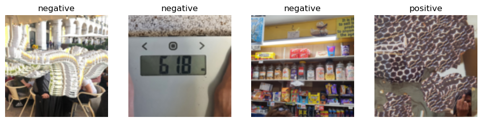
All looking good so far. At the moment the data_block just has each image cropped at a random position, at 128 pixels by 128 pixels. Now lets take a look at some of the different ways we could transform our data, before we use it to train our model.

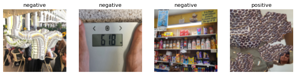
Here’s how it looks with the images ‘squished’:

data_block = data_block.new(item_tfms=Resize(128, ResizeMethod.Squish))
dls = data_block.dataloaders(path/'all')
dls.valid.show_batch(max_n=4, nrows=1)

Here’s how it looks with the images ‘padded’ inorder to fill any space that may be left when minimising them inorder to fit within the specified 128 by 128 size:

data_block = data_block.new(item_tfms=Resize(128, ResizeMethod.Pad, pad_mode='zeros'))
dls = data_block.dataloaders(path/'all',bs=5)
dls.valid.show_batch(max_n=4, nrows=1)

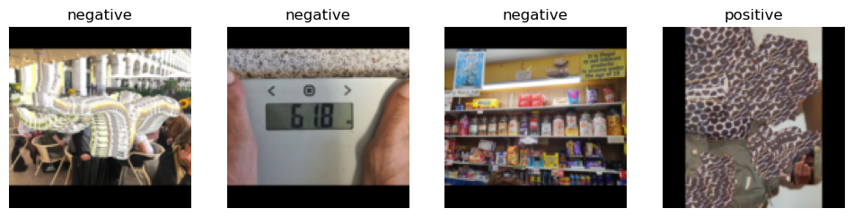
Since the actual image in my image library that I am looking for is not skewed or stretched in anyway, I decided to go for the ‘padded’ mode with my data.

Note how this time I included bs=5 in the dataloaders method call. Without this i kept getting nan for my train_loss when training the model. The following three lines of code were what I used to help me detect what was wrong here:
x,y = learn.dls.one_batch()
out = learn.model(x)
learn.loss_func(out, y)
which gave the error message: ValueError: This DataLoader does not contain any batches.
The debugging code was suggested by KevinB in the first page of this thread on the fastai forum

# x,y = learn.dls.one_batch()
# out = learn.model(x)
# learn.loss_func(out, y)

I then proceeded to train a resnet18 model on my data using vision_learner:

Note before successfully doing so it turned out that I had to downgrade my version of torchvision to 0.12 so that the methods I was opting to use, would work. I also had to upgrade my MacOS operating system as all apple silicon running on anything below 12.3 MacOS did not have Pytorch GPU support.

#!!!ACTIVATE CORRECT ENVIRONMENT BEFORE RUNNING THIS CELL!!!#

# !pip install --upgrade torchvision==0.12

learn = vision_learner(dls, resnet18, metrics=error_rate)
learn.fine_tune(10)

epoch	train_loss	valid_loss	error_rate	time
0	1.761049	2.855227	0.833333	00:03

epoch	train_loss	valid_loss	error_rate	time
0	1.013831	2.266986	0.666667	00:02
1	0.923140	1.505093	0.666667	00:02
2	1.193987	1.579342	0.500000	00:02
3	1.121834	1.969770	0.500000	00:02
4	1.127938	2.468466	0.666667	00:02
5	1.091505	2.685832	0.833333	00:02
6	1.096134	2.706148	0.833333	00:02
7	1.015126	2.648789	0.833333	00:02
8	0.935627	2.475007	0.833333	00:02
9	0.947918	2.624727	0.833333	00:02

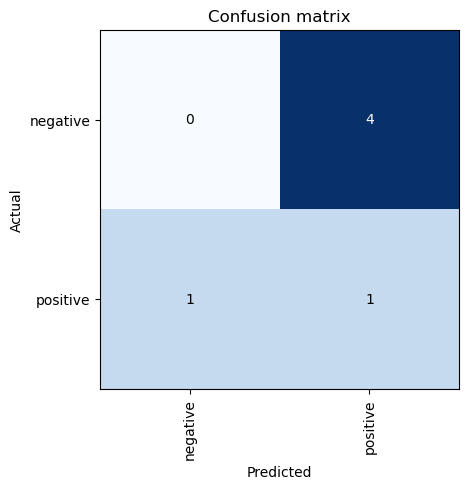
A very underwhelming result, just like in the first method via my simple_net.

Non the less I thought I would confirm just how confused this model is by plotting a confusion matrix:

interp = ClassificationInterpretation.from_learner(learn)
interp.plot_confusion_matrix()

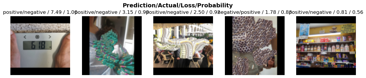
Why not take a look at the top losses whilst were at it!

interp.plot_top_losses(5, nrows=1)

Conclusion

I can only conclude that I, thus far, am using models that are not sufficient for the purpose that I require them for (object detection). I clearly have a lot more to learn about different neural networks and will endeavour to pay close attention to this matter in my continued study.