Gurtaj's blog!

Introduction

Previously I have attempted several different models for tackling this MNIST digit recognition problem (see the Kaggle competition here). The best model I had so far was the most recent which used PyTorch’s nn.Conv2d to manually construct a CNN architecture.

In this notebook I will attempt to create a model using all of the tools available from the fastai library, vision_learner being one of those. I will also use a pretrained model resnet18. There are certainly better models out there, at the time of writing this, but I know this one to be quickly trainable as well as successful on recognising images that are far more complex then black and white hand written digits.

Let’s begin by setting thing’s up in this notebook..

# This Python 3 environment comes with many helpful analytics libraries installed
# It is defined by the kaggle/python Docker image: https://github.com/kaggle/docker-python
# For example, here's several helpful packages to load

import numpy as np # linear algebra
import pandas as pd # data processing, CSV file I/O (e.g. pd.read_csv)

# Input data files are available in the read-only "../input/" directory
# For example, running this (by clicking run or pressing Shift+Enter) will list all files under the input directory

import os
for dirname, _, filenames in os.walk('/kaggle/input'):
    for filename in filenames:
        print(os.path.join(dirname, filename))

# You can write up to 20GB to the current directory (/kaggle/working/) that gets preserved as output when you create a version using "Save & Run All" 
# You can also write temporary files to /kaggle/temp/, but they won't be saved outside of the current session

# install fastkaggle if not available
try: import fastkaggle
except ModuleNotFoundError:
    !pip install -Uq fastkaggle

from fastkaggle import *

setup_comp is from fastkaggle library, it get’s the path to the data for competition. If not on kaggle it will: download it, and also it will install any of the modules passed to it as strings.

comp = 'digit-recognizer'

path = setup_comp(comp, install='fastai "timm>=0.6.2.dev0"')

from fastai.vision.all import *

let’s check whats in the data.

path.ls()

(#3) [Path('digit-recognizer/test.csv'),Path('digit-recognizer/train.csv'),Path('digit-recognizer/sample_submission.csv')]

We have a train.csv and a test.csv. test.csv is what we use for submission. So it looks like we will be creating our validation set, as well as the training set, from train.csv.

let’s look at the data.

df = pd.read_csv(path/'train.csv')
df

	label	pixel0	pixel1	pixel2	pixel3	pixel4	pixel5	pixel6	pixel7	pixel8	...	pixel774	pixel775	pixel776	pixel777	pixel778	pixel779	pixel780	pixel781	pixel782	pixel783
0	1	0	0	0	0	0	0	0	0	0	...	0	0	0	0	0	0	0	0	0	0
1	0	0	0	0	0	0	0	0	0	0	...	0	0	0	0	0	0	0	0	0	0
2	1	0	0	0	0	0	0	0	0	0	...	0	0	0	0	0	0	0	0	0	0
3	4	0	0	0	0	0	0	0	0	0	...	0	0	0	0	0	0	0	0	0	0
4	0	0	0	0	0	0	0	0	0	0	...	0	0	0	0	0	0	0	0	0	0
...	...	...	...	...	...	...	...	...	...	...	...	...	...	...	...	...	...	...	...	...	...
41995	0	0	0	0	0	0	0	0	0	0	...	0	0	0	0	0	0	0	0	0	0
41996	1	0	0	0	0	0	0	0	0	0	...	0	0	0	0	0	0	0	0	0	0
41997	7	0	0	0	0	0	0	0	0	0	...	0	0	0	0	0	0	0	0	0	0
41998	6	0	0	0	0	0	0	0	0	0	...	0	0	0	0	0	0	0	0	0	0
41999	9	0	0	0	0	0	0	0	0	0	...	0	0	0	0	0	0	0	0	0	0

42000 rows × 785 columns

It is just as described in the competition guidelines.

Data Preperation

Lets split this data into training and validation data.
We will split by rows.
We will use 80% for training and 20% for validation. 80% of 42,000 is 33,600 so that will be our split index.

train_data_split = df.iloc[:33_600,:]
valid_data_split = df.iloc[33_600:,:]

len(train_data_split)/42000,len(valid_data_split)/42000

(0.8, 0.2)

Our pixel values can be anywhere between 0 and 255. For good practice, and ease of use later, we’ll normalise all these values by dividing by 255 so that they are all values between 0 and 1.

pixel_value_columns = train_data_split.iloc[:,1:]
label_value_column = train_data_split.iloc[:,:1]

pixel_value_columns = pixel_value_columns.apply(lambda x: x/255)
train_data = pd.concat([label_value_column, pixel_value_columns], axis=1)

train_data.describe()

	label	pixel0	pixel1	pixel2	pixel3	pixel4	pixel5	pixel6	pixel7	pixel8	...	pixel774	pixel775	pixel776	pixel777	pixel778	pixel779	pixel780	pixel781	pixel782	pixel783
count	33600.000000	33600.0	33600.0	33600.0	33600.0	33600.0	33600.0	33600.0	33600.0	33600.0	...	33600.000000	33600.000000	33600.000000	33600.000000	33600.000000	33600.000000	33600.0	33600.0	33600.0	33600.0
mean	4.459881	0.0	0.0	0.0	0.0	0.0	0.0	0.0	0.0	0.0	...	0.000801	0.000454	0.000255	0.000086	0.000037	0.000007	0.0	0.0	0.0	0.0
std	2.885525	0.0	0.0	0.0	0.0	0.0	0.0	0.0	0.0	0.0	...	0.024084	0.017751	0.013733	0.007516	0.005349	0.001326	0.0	0.0	0.0	0.0
min	0.000000	0.0	0.0	0.0	0.0	0.0	0.0	0.0	0.0	0.0	...	0.000000	0.000000	0.000000	0.000000	0.000000	0.000000	0.0	0.0	0.0	0.0
25%	2.000000	0.0	0.0	0.0	0.0	0.0	0.0	0.0	0.0	0.0	...	0.000000	0.000000	0.000000	0.000000	0.000000	0.000000	0.0	0.0	0.0	0.0
50%	4.000000	0.0	0.0	0.0	0.0	0.0	0.0	0.0	0.0	0.0	...	0.000000	0.000000	0.000000	0.000000	0.000000	0.000000	0.0	0.0	0.0	0.0
75%	7.000000	0.0	0.0	0.0	0.0	0.0	0.0	0.0	0.0	0.0	...	0.000000	0.000000	0.000000	0.000000	0.000000	0.000000	0.0	0.0	0.0	0.0
max	9.000000	0.0	0.0	0.0	0.0	0.0	0.0	0.0	0.0	0.0	...	0.996078	0.996078	0.992157	0.992157	0.956863	0.243137	0.0	0.0	0.0	0.0

8 rows × 785 columns

Let’s further process our data so that it is ready for this new type of model we are using. Note that:

• we will use 28*28 pixel matrices for our images rather than 783 pixel vectors
  • because convolutions are done on matrices
• we also add a dimension of 1 as the first dimension (view(1,28,28)) because Conv2d takes in ‘channels’ for each image
  • 3d images would have 2 channels, 1 for each colour (RGB).
  • since we are only dealing with black and white images (one colour) we will deal with only one channel

pixel_value_columns = train_data_split.iloc[:,1:]
label_value_column = train_data_split.iloc[:,:1]

pixel_value_columns = pixel_value_columns.apply(lambda x: x/255)

pixel_value_columns_tensor = torch.tensor(train_data.iloc[:,1:].values).float()
# here we change from image vectors to image matrices (via `.view`) and put it in our three channels (via `.expand`) ( we want three channels since resnet18 expects 3 channel images (RGB))
pixel_value_matrices_tensor = [row.view(28,28).expand(3,28,28) for row in pixel_value_columns_tensor]

label_value_column_tensor = torch.tensor(train_data.iloc[:,:1].values).float()

# F.cross_entropy requires that the labels are tensor of scalar. label values cannot be `FloatTensor` if they are classes (discrete values), must be cast to `LongTensor` (`LongTensor` is synonymous with integer)
train_ds = list(zip(pixel_value_matrices_tensor, label_value_column_tensor.squeeze().type(torch.LongTensor)))

train_dl = DataLoader(train_ds, batch_size=256)

Lets do the same for the validation data.

pixel_value_columns = valid_data_split.iloc[:,1:]
label_value_column = valid_data_split.iloc[:,:1]

pixel_value_columns = pixel_value_columns.apply(lambda x: x/255)

pixel_value_columns_tensor = torch.tensor(train_data.iloc[:,1:].values).float()
    # NOTE how in .expand we can use `-1` instead of `28` to say 'keep this dimension the same size as it is originally'
pixel_value_matrices_tensor = [row.view(28,28).expand(3,-1,-1) for row in pixel_value_columns_tensor]

label_value_column_tensor = torch.tensor(train_data.iloc[:,:1].values).float()

valid_ds = list(zip(pixel_value_matrices_tensor, label_value_column_tensor.squeeze().type(torch.LongTensor)))

valid_dl = DataLoader(valid_ds, batch_size=256)

dls = DataLoaders(train_dl,valid_dl)

Let’s see if we now have the format we need.

valid_xb,valid_yb = first(valid_dl)
valid_xb.shape,valid_yb.shape

(torch.Size([256, 3, 28, 28]), torch.Size([256]))

So we have:

• tuples of (x, y),
• and for x we have
  • batches of 256,
  • images of 3 channels (even though it is a black and white image we tripled the channels as resnet18 works with RGB/3-channel images),
  • of size 28 by 28 pixels.
• and for y we have
  • batches of 256 of,
  • single values (the ground truth/digit label).

NOTE: that the way in which we trippled our channels was very inneficient. First we converted them to numpy arrays inorder to change their combination back to a tensor in the end. There must be a more efficient way of doing this that I am yet to learn.

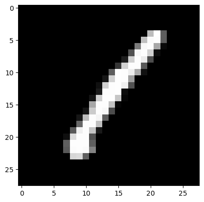
To ease my mind and help spot places where I could be making errors, i’ll make a function that can visually show a particular input (digit image) to me.

def show_image(item):
    plt.gray()
    plt.imshow(item, interpolation='nearest')
    plt.show()

# we access the first channel of the first image of our first batch of validation data
show_image(valid_xb[0][0])

Model Creation and Training

Now let’s see what we can do with this data using resnet18 architecture CNN model with fastai’s vision_learner.

Note that we will also use fine_tune here rather than fit or fit_one_cycle since we don’t want to retrain the whole model, just the head (last layers) in order to utilise its pre-existing trained wieghts but then specify their use towards our specific goal.

learn = vision_learner(dls, resnet18, metrics=accuracy, n_out=10, normalize=False, loss_func=F.cross_entropy)

learn.fine_tune(1)

epoch	train_loss	valid_loss	accuracy	time
0	1.278895	0.619535	0.802321	06:30

epoch	train_loss	valid_loss	accuracy	time
0	0.268740	0.103634	0.968423	12:43

0.968423 sounds like a very good accuracy indeed. But, going off previous attempts, this is not reason alone to get excited and start expecting a great result on the leaderbaord. The only way to gauge that will be to make a submission, so let’s do that!

Submitting Results

First let’s pre process the test data like we did with our training data, since this is how our model expects it.

test_df = pd.read_csv(path/'test.csv')
test_df.describe()

	pixel0	pixel1	pixel2	pixel3	pixel4	pixel5	pixel6	pixel7	pixel8	pixel9	...	pixel774	pixel775	pixel776	pixel777	pixel778	pixel779	pixel780	pixel781	pixel782	pixel783
count	28000.0	28000.0	28000.0	28000.0	28000.0	28000.0	28000.0	28000.0	28000.0	28000.0	...	28000.000000	28000.000000	28000.000000	28000.000000	28000.000000	28000.0	28000.0	28000.0	28000.0	28000.0
mean	0.0	0.0	0.0	0.0	0.0	0.0	0.0	0.0	0.0	0.0	...	0.164607	0.073214	0.028036	0.011250	0.006536	0.0	0.0	0.0	0.0	0.0
std	0.0	0.0	0.0	0.0	0.0	0.0	0.0	0.0	0.0	0.0	...	5.473293	3.616811	1.813602	1.205211	0.807475	0.0	0.0	0.0	0.0	0.0
min	0.0	0.0	0.0	0.0	0.0	0.0	0.0	0.0	0.0	0.0	...	0.000000	0.000000	0.000000	0.000000	0.000000	0.0	0.0	0.0	0.0	0.0
25%	0.0	0.0	0.0	0.0	0.0	0.0	0.0	0.0	0.0	0.0	...	0.000000	0.000000	0.000000	0.000000	0.000000	0.0	0.0	0.0	0.0	0.0
50%	0.0	0.0	0.0	0.0	0.0	0.0	0.0	0.0	0.0	0.0	...	0.000000	0.000000	0.000000	0.000000	0.000000	0.0	0.0	0.0	0.0	0.0
75%	0.0	0.0	0.0	0.0	0.0	0.0	0.0	0.0	0.0	0.0	...	0.000000	0.000000	0.000000	0.000000	0.000000	0.0	0.0	0.0	0.0	0.0
max	0.0	0.0	0.0	0.0	0.0	0.0	0.0	0.0	0.0	0.0	...	253.000000	254.000000	193.000000	187.000000	119.000000	0.0	0.0	0.0	0.0	0.0

8 rows × 784 columns

Like our traning data, the test data has values for each pixel in each image. Unlike our test data it does not include any labels for any of the images. Therefore our data preperation will take this difference into account. We will create a DataLoader in order to feed our data into the model but we since DataLoaders require labels and we don’t have any, we will just create some dummy 0 value labels instead.

def dataloader_from_test_dataframe(dframe):
    pixel_value_columns = dframe.apply(lambda x: x/255)

    pixel_value_columns_tensor = torch.tensor(pixel_value_columns.values).float()
    pixel_value_matrices_tensor = [row.view(28,28).expand(3,-1,-1) for row in pixel_value_columns_tensor]

    dummy_label_value_column_tensor = torch.zeros(len(pixel_value_columns_tensor)).float()

    ds = list(zip(pixel_value_matrices_tensor, dummy_label_value_column_tensor.squeeze().type(torch.LongTensor)))

    return DataLoader(ds, batch_size=len(pixel_value_columns_tensor))

test_dl = dataloader_from_test_dataframe(test_df)

test_xb,test_yb = first(test_dl)
test_xb.shape,test_yb.shape

(torch.Size([28000, 3, 28, 28]), torch.Size([28000]))

show_image(test_xb[0][0]),show_image(test_xb[1][0])

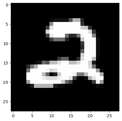
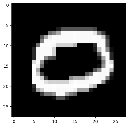
(None, None)

Notice how we didn’t include the final step of creating a dataloader here, like we did for our training and validation data earlier. That’s because, for some reason, we now need to use the test_dl method on the dls object of our learn. I think it is something to do with how I have done this all manaully in a way that we normally wouldn’t in real practice. (for the sake of learning). For example there is the fact that I earlier used DataLoader on the training and validation data instead of ImageDataLoaders or DataBlock with the appropriate input and output types declared (ImageBlock and CategoryBlock respectively).

The methods used below were acquired from this comment in the fastai forums.

preds = learn.get_preds(dl=test_dl)

preds_x,preds_y = preds
preds_x.shape,preds_y.shape

(torch.Size([28000, 10]), torch.Size([28000]))

We are getting tuples as our output. The first item in each tuple is the activation that corresponds to each possible class that we are classifying our inputs by (each possible digit). The second item in the tuple is just always 0 as this is the dummy label we added to our DataLoader. Let’s confirm by looking at a few.

preds_x[0],preds_y[0],preds_x[1],preds_y[1],preds_x[2],preds_y[2],preds_x[3],preds_y[3],preds_x[4],preds_y[4]

(tensor([-2.1849, -0.6895, 13.6192,  4.5025, -4.8089,  3.7261, -5.1013, -3.5475,
         -0.4706, -3.9076]),
 tensor(0),
 tensor([ 7.8694, -2.0303, -3.1039, -1.5830, -1.8573, -2.4699,  0.6730, -2.8973,
         -0.3747,  0.0887]),
 tensor(0),
 tensor([-2.2344, -3.3648, -0.4304,  0.4682, -3.0089,  1.7690, -1.3859, -2.9892,
          5.0062,  2.8473]),
 tensor(0),
 tensor([ 0.2836, -2.3423,  1.0665,  1.1372, -2.7025,  2.5808,  2.2428, -2.8127,
          1.8188, -1.4930]),
 tensor(0),
 tensor([-4.4768, -2.5752,  3.9028, 12.8070, -2.8616,  2.3295, -2.0011, -2.2258,
         -2.3868, -3.6948]),
 tensor(0))

The negative activation values are throwing me off as I did not expect it, non the less I will go ahead and take the index of the highes activation value in each prediction, as our predicted class.

def get_predicted_label(pred):
    #returns index of highest value in tensor, which convenietnly also is directly the the digit/label that it corresponds to
    return torch.argmax(pred)

# .numpy() turns the scalar tensors into normal scalar variable in python
predictions_list = [get_predicted_label(pred).numpy() for pred in preds_x]

predictions_list[:5]

[array(2), array(0), array(8), array(5), array(3)]

pred_labels = pd.Series(predictions_list, name="Label")

pred_labels

0        2
1        0
2        8
3        5
4        3
        ..
27995    9
27996    7
27997    3
27998    9
27999    2
Name: Label, Length: 28000, dtype: object

ss = pd.read_csv(path/'sample_submission.csv')

ss

	ImageId	Label
0	1	0
1	2	0
2	3	0
3	4	0
4	5	0
...	...	...
27995	27996	0
27996	27997	0
27997	27998	0
27998	27999	0
27999	28000	0

28000 rows × 2 columns

ss['Label'] = pred_labels

ss

	ImageId	Label
0	1	2
1	2	0
2	3	8
3	4	5
4	5	3
...	...	...
27995	27996	9
27996	27997	7
27997	27998	3
27998	27999	9
27999	28000	2

28000 rows × 2 columns

Looks good! now we can submit this to kaggle.

We can do it straight from this note book if we are running it on Kaggle, otherwise we can use the API
In this case I did it directly using the kaggle notebook UI and selecting my ‘subm.csv’ file from the output folder there (see these guidelines)

# this outputs the actual file
ss.to_csv('subm.csv', index=False)
#this shows the head (first few lines)
!head subm.csv

ImageId,Label
1,2
2,0
3,8
4,5
5,3
6,7
7,0
8,3
9,0

!kaggle competitions submit -c digit-recognizer  -f ./subm.csv -m "vision learner"

This got a score of 0.9471 which is just the tiniest bit below the score we got for the CNN we made by manually constructing our architecture using PyTorch module nn.Conv2d (see the previous notebook)

Conclusion

fastai’s vision_learner and fine_tune, allowed us the benefit of using a pre-made, tried and proven, architecture, along with its pre-learned weights.

With singificantly less training time than that which was required for the previous nn.Conv2d model, and still receiving almost the same score, it can be seen that using vision_learner has improved our efficiency by a great deal.